Security of machine learning algorithms. Python attacks

Machine learning is actively used in many areas of our life. Algorithms help recognize traffic signs, filter spam, recognize faces of our friends on facebook, even help them trade on stock exchanges. The algorithm makes important decisions, so you need to be sure that it can not be deceived.
In this article, which is the first of a series, we will introduce you to the problem of the safety of machine learning algorithms. This does not require a high level of machine learning knowledge from the reader; it is enough to have a general idea of this field.
First, we give the terms used in the subject of security of machine learning algorithms:
Adversarial example is a vector applied to the algorithm on which the algorithm gives an incorrect output.
Adversarial attack is an algorithm of actions whose goal is to obtain an Adversarial example.
To understand the problem of Adversarial examples, let us recall one of the tasks of machine learning - learning with a teacher in classifying. In this problem, we have the object-tag pairs, and we must learn to predict the value for new objects.
If we consider this problem from a geometrical point of view, then it is necessary to divide the space in such a way that to predict the “correct” class on the new object. Moreover, if we had a general set of data (for example, for a set of MNIST handwritten digits to have all sorts of images of all digits), then this hyperplane could be carried out ideally, provided that the classes are separable. But since the general totality most often does not happen, then we use machine learning algorithms to solve this problem — in order to bring the “ideal” hyperplane as accurately as possible using the data that we have.
Any deviation of the hyperplane from the ideal, generates some “gap”, falling into which, the objects are classified incorrectly. That is why there are such examples as the panda, classified as a gibbon. And the attacker's task is to change the vector of the object's parameters in such a way that it falls into this “gap”.
Examples of Adversarial Attacks
There is a neural network that detects the face in the photo. She successfully copes with the task (image on the left). But after adding a slight noise to this photo (image on the right), the algorithm in the resulting adversarial example (image in the center) no longer detects the face in the image.
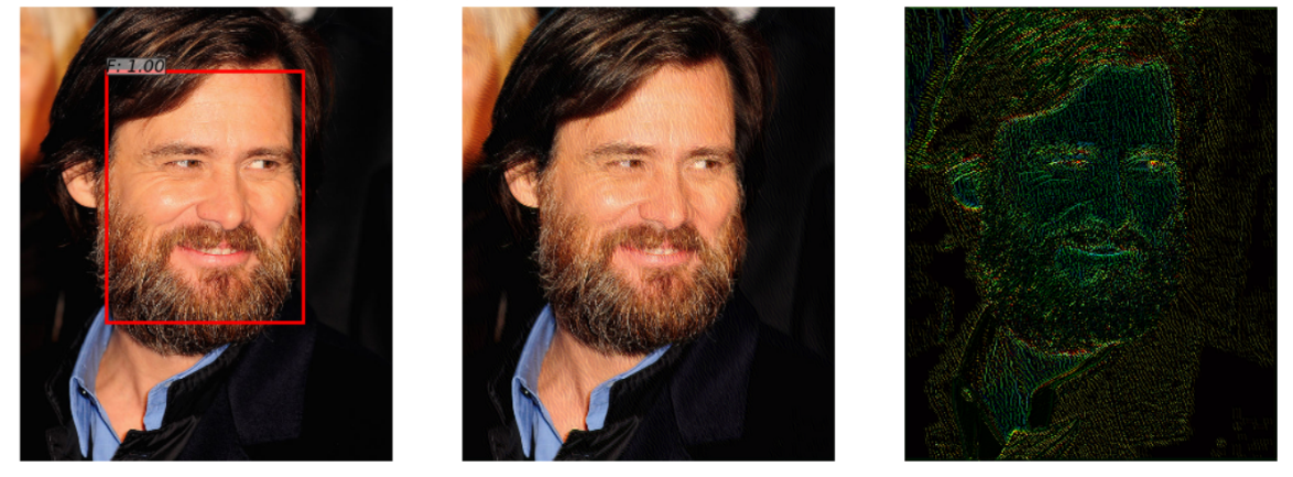
This example, demonstrated in the article “ Adversarial Attacks on Face Detectors using Neural Net Based Constrained Optimization ”, is interesting because a lot of real face recognition systems use neural network approaches to detect faces. A person will not notice the difference when looking at both images.
The following example was taken from the automotive, namely, the recognition of road signs. This example is interesting because the adversarial example does not have to be an object at least somewhat close to the objects on which the network was trained. For example, in “ Rogue Signs: Deceiving Traffic Sign Recognition with Malicious Ads and Logos ”, it was shown that the resulting adversarial example of the KFC sign would be “recognized” by the original neural network as a STOP sign with a 100% probability.

Many could doubt the use of adversarial examples in the real world, since previous examples were tested on a computer, whereas in real life such an object is hardly possible to obtain. But it is not. In " Synthesizing Robust Adversarial Examples ", it was shown that the adversarial example made on a computer can be successfully printed on a 3D printer, and the algorithm will make the same mistakes as in a computer simulation.
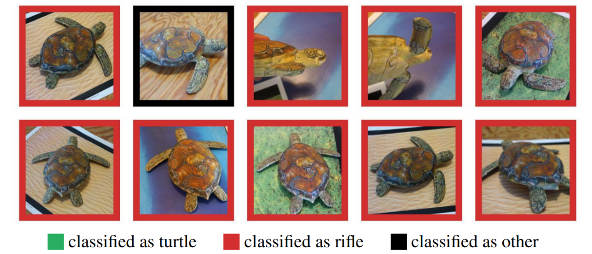
Here you see a turtle printed on a 3D printer that was not recognized as a turtle at any angle.
The following example shows what can be done if we go beyond the usual understanding of the adversarial attack. Namely, reprogram the source network to use its own payload. In other words, we learn to use someone else’s neural network to solve the problem posed by the attacker. For example, Adversrial Reprogramming of Neural Network demonstrated how the network trained on ImageNet perfectly counted the number of squares in the image and recognized the digits from the MNIST set.
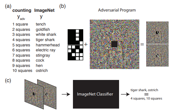
The picture shows the algorithm of Adversarial Reprogramming, which is recommended to get acquainted with in the original article.
In this article I would like to talk about how to generate Adversarial examples, and in the second article we will move on to ways to protect and test machine learning algorithms.
Attack classification
All attacks can be divided into 2 classes: WhiteBox (WB) and BlackBox (BB) . In the case of WB, we know all the information about the trained model of the algorithm, whereas in the case of BB, we have access only to the input and output of the model. In fact, the GrayBox option is still possible when we do not know the information about the trained model, but there is information about the type of the algorithm and its hyperparameters. But this type is not allocated in a separate class, as additional information is not enough to go to WB, which means it is just an additional set of information for conducting a BB attack.
Next is to classify attacks on Targeted and Non Targeted . Targeted attacks imply that an attack takes place in a certain direction. For example, on the MNIST dataset, we will train the neural network and take image 0 from the test set. The trained neural network gives the class 0 probability in this object equal to 1.00. If we want the adversarial example to be recognized as class 1 after applying the adversarial attack, then we will apply the Targeted attack. Otherwise, if it is not very important for us what class the neural network will take the resulting image (the main thing is that it is no longer class 0), then such an attack will be Non Targeted.
In addition, attacks are divided into a metric, according to which 2 objects are considered similar - norms. the norm is the number of parameters changed. Euclidean distance between two vectors. maximum elementwise difference between two vectors.
Python libraries
These Python libraries allow you to work with Adversarial examples. These are FoolBox, CleverHans and ART-IBM.
| Foolbox | Cleverhans | ART-IBM | |
|---|---|---|---|
| Supported frameworks | TensorFlow, Keras, Theano, PyTorch, Lasagne, MXNet | TensorFlow, Keras | TensorFlow, Keras, promise MXNet, PyTorch |
Now let's take a closer look at the attacks, and start with the WhiteBox attacks.
L-BFGS attack
The formulation of the L-BFGS method can be written with the following formula.
From this it follows that we want to minimize the loss function in the direction of the target class with the restriction that the changes made are minimal. In this case, to solve such a problem in the original article was proposed precisely using the L-BFGS method, hence the name of this attack.
Original article - Intriguing properties of neural networks
This attack is presented in 2 of 3 previously announced libraries - FoolBox and CleverHans.
And the use of this attack on FoolBox takes 3 lines of Python code:
from foolbox.attacks import LBFGSAttack
attack = LBFGSAttack(fmodel)
adversarial = attack(image, label)
Using L-BFGS will help you find the best adversarial examples based on your limitations, but, firstly, the search for such an example can take a long time, and, secondly, it is quite possible that the method simply does not converge.
FGSM attack
The next stage of development was the FGSM (Fast Sign Gradient Method) method, which can be shown using the formula:
This method works much faster than L-BFGS. Here we simply take the signs from the gradient function of the original loss function, multiplying the sign by someadd to the original image.

Here is an example of how this method works. The noise map with equal to 0.007, and it turns out that the photo of the panda is now recognized as a Gibbon with a probability of 99.3%
This method is notable for simplicity of implementation, but at the same time, the result of the work of this method is very noisy.
Original article - Explaining and Harnessing Adversarial Examples
You can find the implementation of this method in libraries, and using it on the foolbox will also not take long
from foolbox.attacks import FGSM
attack = FGSM(fmodel)
adversarial = attack(image, label)
DeepFool attack
DeepFool is a Non Targeted method. Its main difference from the previous methods is that it tries to make a minimal noise map that will deceive the algorithm. The method does not allow you to make one particular class from one class, but does any other that is closest to the original image.
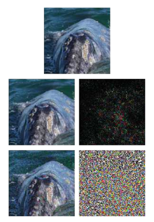
The example shows the source image, on the bottom line - the FGSM method, and in the middle - just DeepFool attack. It can be seen that the noise map is much smaller than with FGSM.
Original article - DeepFool: fool deep neural networks
Such an attack can be performed using any of the listed libraries, and the implementation on ART-IBM takes only 3 lines of code:
from art.attacks import DeepFool
attack = DeepFool(model)
img_adv = attack.generate(img)
Jacobian saliency map attack
In the JSMA method, the direct derivative is considered, on the basis of which the gradient map is constructed. On the map, in fact, each parameter of the object corresponds to the contribution of this parameter to the change in the final result of the algorithm. Thus, the method allows changing as few parameters as possible in the attacked object. And, accordingly, it works by norm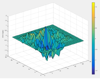
Original article - The Limitations of Deep Learning in Adversarial Settings
This attack can be carried out using CleverHans or ART-IBM. And on CleverHans it looks like this:
from cleverhans.attacks import SaliencyMapMethod
jsma = SaliencyMapMethod(model, sees=sees)
jsma_params = { 'theta' : 1., 'gamma' : 0.1,
                            'clip_min' : 0., 'clip_max' : 1.,
                            'y_target' : None}
adv_x = jsma.generate_np(img, **jsma_params)
One pixel attack
The logical question is, what minimum number of pixels must be changed in order to attack the algorithm, and as many have already guessed from the name of the attack, 1 pixel is enough.

For example, an image of a horse with just one modified pixel becomes a frog with a probability of 99.9%
Original article - One pixel attack for fooling deep neural networks
This attack is supported only in FoolBox, and its conduct is as follows:
from foolbox.attacks import SinglePixelAttack
attack = SinglePixelAttack(fmodel)
adversarial = attack(image,max_pixel=1)
It is worth making a reservation and saying that the implementation of the algorithm in Foolbox, compared to the original article, although it has a common goal (to change a specific number of pixels in the image), but differs in the method of obtaining the image.
Methods based on the generalization of the BlackBox model
Most of the methods require an understanding of how the architecture of the model is arranged, knowledge of the exact values of its parameters, but in practice this is quite rare. And that is why a separate attack direction appears - BlacBox / GrayBox attacks. For such attacks, it is enough to have access to the input and output of the model.
One of the methods for realizing an attack on the BlackBox model is a generalization of this model to the Student (in the Substitute picture) model.
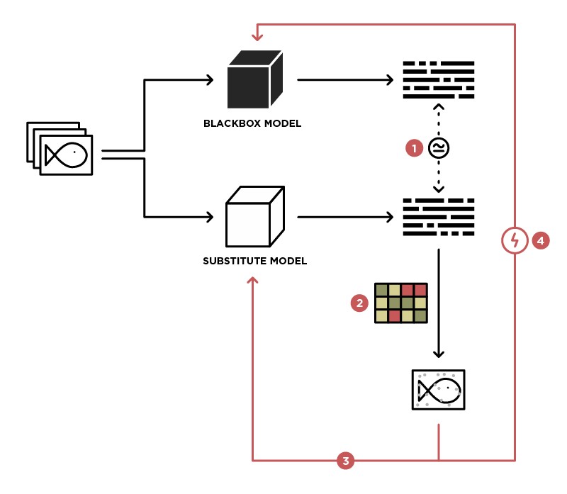
Having access to sending data to the BlackBox model (Teacher) and access to the output of this model, we can form a dataset on which it is possible to train our own model (Student), thereby summarizing the Teacher model. After that, you can use the WhiteBox attack on the Student model, and most likely this attack will take place on the Teacher model. The probability of such an attack is the higher, the more knowledge about the Teacher model we have. For example, we know that the Teacher model handles images; most often, pre-trained architectures (ResNet, Inception) with ImageNet weights are used for image processing. Taking Student model with the same architecture as a basis, the probability of a successful attack will be maximal.
Original article - Practical Black-Box Attacks against Machine Learning
This method is not represented in any of the libraries and requires self-implementation of the Student model, and attacks on it can be carried out using the methods described above.
GAN-based methods
The next stage in the development of the BlackBox attacks was attacks based on embedding the BlackBox model into the Generative-Competitive Network (GAN) architecture, a network that allows you to generate new objects that will later be transferred to the Black-Box model.

This method allowed us to generate adversarial examples for almost any architecture. His work also requires access to the input and output of the attacked model.
You can read more about this method in the original article - UPSET and ANGRI: Breaking High Performance Image Classifiers
As you might have guessed, these methods are not represented in any of the libraries.
Conclusion
In fact, there are a large number of attacks. This article covers only some of them. We hope that this material has helped you to understand the basic concepts of adversarial examples and algorithms for their generation. For more detailed acquaintance we recommend to get acquainted with original articles and materials from the list of references.
See you in the next article, where we will talk about the methods of protection and testing of machine learning algorithms.
Bibliography
- Threat of Adversarial Attacks on Deep Vision: A Survey - a great overview of attack methods on deep learning algorithms in the Computer Vision task
- Attacking Machine Learning with Adversarial Examples - OpenAI's blog on adversarial examples
- Awesome Adversarial Machine Learning - a githab with links to many useful Adversarial topics
- Adversarial Machine Learning Presentation - Presentation from the MoscowPythonConf2018 Conference on Adversarial Machine Learning
