Sum of arithmetic progressions

We need to find out how many options for the location of occupied cells exist.
A lot of tasks come down to this scheme. For example, dividing a period of N + 1 calendar days into l + 1 consecutive smaller periods. Suppose we want to carry out an optimization calculation using the “brute force” method, calculating the objective function for each possible variant of the period splitting, in order to choose the best option. To estimate the calculation time in advance, you need to determine the number of options. This will help to decide whether to start the calculation at all. Agree - it will be useful to warn the user of your program in advance that with the parameters that he set, the calculation will take 10,000 years.
There is a simple formula that allows for any N and l to get the number of all possible options for the location of occupied cells:


This is the formula for the sum of the sums of the sums ... the sums of arithmetic progressions of the form 1 + 2 + 3 + ... + n; the word "sum" in different declensions in this phrase is repeated exactly l - 1 time. In other words, this formula allows you to quickly calculate these amounts:

An ordinary desktop PC takes too much time to calculate these amounts “head-on” (especially using long arithmetic - and you can’t do without it).
When I was just starting to solve this problem (and I did not know this formula yet), I scored the phrase “sum of arithmetic progressions” into the search engine and did not find anything. That is exactly what I called my article - with the expectation that the next seeker of this formula can quickly find it here.
I have no links to an authoritative source regarding this formula. I deduced it analytically and checked numerically, having conducted over 4000 tests. If you are interested, its conclusion is given at the end of the article.
Soon I will tell you how arithmetic progressions are related to counting cell layout options, but for now I’ll give you some more ready-made formulas.
We introduce an additional condition: suppose, in any scenario, there must be at least 1 group of r adjacent unoccupied cells. In this case, the number of options is determined as follows:
![$ S_l ^ r (n) = (l + 1) \ cdot S_l (nr) - \ sum_ {j = 0} ^ {l-1} \ sum_ {i = r} ^ {nr-1} \ left [S_j ^ r (i + 1) \ cdot S_ {lj-1} (nri) \ right] $](https://habrastorage.org/getpro/habr/formulas/ede/71c/5d1/ede71c5d1e9cc69aca086c00d08d10dc.svg)


If your program performs any calculations for each cell layout option, then the calculations for different options are probably the same. This means that they are easily distributed across multiple threads. The article will tell you how to organize iteration over options so that each thread gets an equal number of options.
1. And where does the progression?
This is the easiest question. Group all the occupied cells at the left end of your row of cells - so that they follow one after the other, starting from the leftmost cell in the row:

How many options are there for the location of the rightmost of the occupied cells (we will call it the last occupied cell), provided that the remaining cells remain in their places? Exactly n. Now move the PASTLAST-SIZED CELL to the right by 1 position. How many positions are left for the last cell? n - 1. The penultimate cell can be shifted to the right n times. So, there will be so many options for the location of the last two occupied cells: S 2 (n) = 1 + 2 + 3 + ... + n. Move the third occupied cell to the right by 1 position and again count the number of options for the location of the last and penultimate cells. It turns out S 2 (n - 1). The third cell can also be shifted to the right only n times, and in all the options for the location of the last three cells will be S 3 (n) = S 2(1) + S 2 (2) + ... + S 2 (n).
Reasoning this way, we finally get to the number of location options for all l occupied cells:
2. Additional condition: at least 1 group of r unoccupied adjacent cells
First, we consider special cases. If n + l - 1 ≥ r (l + 1), then in no case will we get a variant in which there is at least 1 group of r unoccupied cells. Even in the worst case, when the occupied cells in the row are evenly distributed so that the distance between them and the edges of the row is r - 1, the number of occupied cells is simply not enough for ALL of these distances to be no more than r - 1. At least one will be equal to at least r. Consequently:
If you fix the leftmost occupied cell in the leftmost position, the location options for all other cells will be S r (l - 1) (n). If you move it 1 position to the right, the options will be S r (l - 1) (n - 1). Starting from position r + 1, we will always have a gap of at least r at the left end of the row, so that the rest of the options can be calculated without recursion: S l (n - r). It turns out this:

Now we can move on to distributing iterations over the flows. To understand this, you must clearly understand how the first formula S r l (n) was derived , because This conclusion contains a certain iteration order for the location options of occupied cells.
3. How to organize iteration in multiple threads
The iteration order will be common to all threads. Initially, all l cells are located at the left end of the row, occupying positions 1 through l. This is the first iteration. The extreme right cell at each iteration moves to the right by 1 position until it is at the end of the row, then the cell to the left of it moves 1 position to the right, and the extreme cell again passes all possible positions between the cell to the left and the right end of the row. When both cells are in the far right position, the cell to the left of them moves 1 position to the right. And so on until all the cells are at the right end of the row. In the iteration, we skip options in which there is not a single group of r adjacent unoccupied cells.
According to this iteration order, we select the first k options and assign them to the first thread, then assign the next k options to the second thread, and so on. Suppose we decided to use n t flows, the number of iterations in each of which we determined as k i , i = 1, ..., n t .
The sequence number of the first iteration for each stream is called h i :

using Anylong = boost::multiprecision::cpp_int;
using Opt_UVec = boost::optional<std::vector<unsigned> >;
Opt_UVec arrangement(Anylong index, unsigned n, unsigned l, unsigned r = 0);
The arrangement function accepts the index variant number and row parameters: n = N - l + 1, l and r, - and returns a vector with the positions of the occupied cells in the row. The position of a busy cell is an integer from 1 to N.
The number of options grows very quickly with increasing parameters l and n, so we need a long arithmetic to represent this number. I used the boost :: multiprecision :: cpp_int class , capable of representing integers of any length.
If the index parameter exceeds the number of possible cell locations, the function returns an empty boost :: optional object . If the index parameter or n parameter is 0, this is treated as a programmer error, and the function throws an exception.
First, translate into C ++ formulas to determine the number of options:
structException
{enumclassCode { INVALID_INPUT = 1 } code;
    Exception(Code c) : code(c) {}
    static Exception InvalidInput(){ return Exception(Code::INVALID_INPUT); }
};
Anylong S(unsigned n, unsigned l){
    if (!n) throw Exception::InvalidInput();
    if (l == 1) return n;
    if (n == 1 || l == 0) return1;
    Anylong res = 1;
    for (unsigned i = 1; i <= l; ++i) {
        res = res * (n + i - 1) / i; // порядок действий важен!
    }
    return res;
}
Anylong S(unsigned n, unsigned l, unsigned r){
    if (!n) throw Exception::InvalidInput();
    if (r == 0) return S(n, l);
    if (r == 1) if (n == 1) return0; elsereturn S(n, l);
    if (n + l - 1 >= r * (l + 1)) return S(n, l);
    if (n <= r) return0; elseif (l == 0) return1;
    Anylong res = (l + 1) * S(n - r, l);
    for (unsigned j = 0; j <= l - 1; ++j)
        for (unsigned i = r; i <= n - r - 1; ++i)
            res -= S(i + 1, j, r) * S(n - r - i, l - j - 1);
    return res;
}
Pay attention to this line:
res = res * (n + i - 1) / i;The procedure is important here. The product of the factors res and (n + i - 1) is always divided entirely by i, but each of them individually is not. Violation of the procedure will lead to distortion of the results.
Now a hundred and t questions, how to determine the location option by index.
Recall the iteration order we adopted. To shift the leftmost cell 1 position to the right, X 1 = S r l - 1 (n) iterations will be required . You can move it another 1 cell to the right in X 2 = S r l - 1 (n - 1) iterations. If at some point X 1 + X 2 + ... + X i + X i + 1turned out to be more than index, which means we just determined the position of the first occupied cell. It should be in the i-th position. Next, we calculate how many iterations are required to move the second cell to the right: X 1 = S r l - 2 (n - i + 1). This continues until we get to the option number index. If at least i turned out to be greater than r, all subsequent calls to S r l (n) are replaced by S l (n), because we already have at least one gap of at least r to the left of the current cell.
It will be shorter to write the code than to explain in words.
Opt_UVec arrangement(Anylong index, unsigned n, unsigned l, unsigned r = 0){
    if (index == 0) throw Exception::InvalidInput();
    if (index > S(n, l, r)) return {};
    std::vector<unsigned> oci(l); /* occupied cells indices - позиции
                              занятых ячеек в ряду (индексы от 1 до N) */if (l == 0) return oci;
    if (l == 1) {
        assert(index <= std::numeric_limits<unsigned>::max());
        oci[0] = (unsigned)index;
        return oci;
    }
    oci[0] = 1;
    unsigned N = n + l - 1;
    unsigned prev = 1;
    Anylong i = 0; auto it = oci.begin();
    while (true) {
        auto s = S(n, --l, r);
        while (i + s <= index) {
            if ((i += s) == index) {
                auto it1 = --oci.end();
                if (it1 == it) return oci;
                *it1 = N;
                for (it1--; it1 != it; it1--) *it1 = *(it1 + 1) - 1;
                return oci;
            }
            s = S(--n, l, r);
            assert(n);
            (*it)++;
            if (r && (*it) > prev + r - 1) r = 0;
        }
        prev = *it++;
        assert(it != oci.end());
        *it = prev + 1;
    }
    assert(false);
}
4. Derivation of formulas
I will please fans of school algebra with another section.
Let's start with the sum of the arithmetic progressions:


![$ S_ {l-1} (n) = \ left [\ prod_ {i = 1} ^ {l-1} \ frac {n + i-1} {i} \ right] \ times \ frac {(n + l-1) - (n + 0-1)} {l} $](https://habrastorage.org/getpro/habr/formulas/534/137/6da/5341376dadf8576ce7d6c080c9ba50a7.svg)

Now back to the formula for calculating options for r ≠ 0:
We calculate the number of options when the gap between the last occupied cell and the right end of the row is greater than or equal to r. It is as if the last occupied cell had grown in size to r + 1, while the dimensions of the row would have remained the same:

This number of options is equal to S l (n - r).
Now we add to it the number of options in which the gap between the last and penultimate occupied cells is greater than or equal to r. This number of options will again be equal to S l (n - r). But we already counted some of these options when we calculated the previous S l (n - r). Namely, those variants in which the gap between the last occupied cell and the right end of the row is greater than or equal to r. Therefore, to the first S l (n - r) variants, it is necessary to add not S l (n - r), but S l(n - r) - X, where X is the number of options in which the gap between the last and penultimate occupied cells is greater than or equal to r, as well as the gap between the last occupied cell and the right end of the row.
Exactly the same thing will have to be done for each jth occupied cell - from S l (n - r) subtract X j equal to the number of options in which the gap between the jth cell and the cell to the left of it (in the case of the leftmost cell - the gap between it and the left end of the row), as well as at least one of the gaps to the right of the jth cell, are greater than or equal to r.
In total, we have l - 1 gaps between occupied cells, plus 2 gaps between a busy cell and the end of the row. Therefore, the term S l (n - r) is included in our formula l + 1 times. And here is X jnot calculated for the gap between the rightmost occupied cell and the right end of the row. Hence, these terms will be only l.

Take a look at this picture:
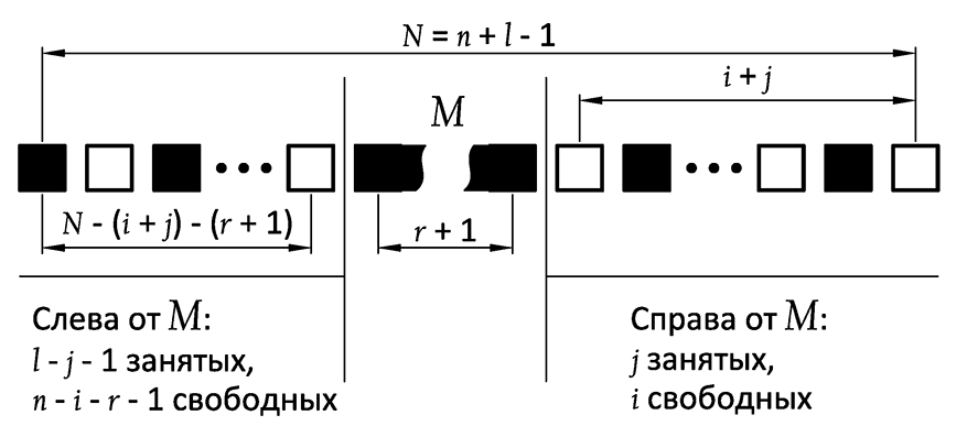
the jth cell (the one that grows to size r + 1 when iterating over j) is denoted as M. It can be in n - r possible positions, which are determined by the parameter i (i ∈ [0, n - r - 1]) . The first r positions can not be considered, since for i <r all the intervals to the right of M will be less than r. Therefore, i ∈ [r, n - r - 1].
The number of cell location options to the right of M in which at least 1 gap is greater than or equal to r is S r j (i + 1). The number of cell location options to the left of M is S l - j - 1 (n - i - r). In total, we obtain S r j (i + 1) ∙ S l - j - 1 (n - i - r) for all i ∈ [r, n - r - 1] and all j ∈ [0, l - 1]: