I work in a team of the Odnoklassniki platform and today I’ll tell you about the architecture, design and implementation details of the music distribution service.

The article is a transcript of the report on Joker 2018 .

Some statistics

First, a few words about OK. This is a giant service that is used by more than 70 million users. They are served by 7 thousand machines in 4 data centers. Recently, on traffic, we broke the 2 TB / s mark without counting numerous CDN sites. We squeeze the maximum out of our hardware, the most loaded services serve up to 100,000 requests per second from a four core node. At the same time, almost all services are written in Java.

In OK, many sections, one of the most popular - "Music". In it, users can upload their tracks, buy and download music in different qualities. In the section there is a wonderful catalog, recommendation system, radio and much more. But the main purpose of the service, of course, is playing music.

The distributor of music is engaged in data transfer to user players and mobile applications. It can be caught in the web inspector, if you look at requests to the domain musicd.mycdn.me. API distributor is extremely simple. It responds to HTTP requests GETand issues the requested track range.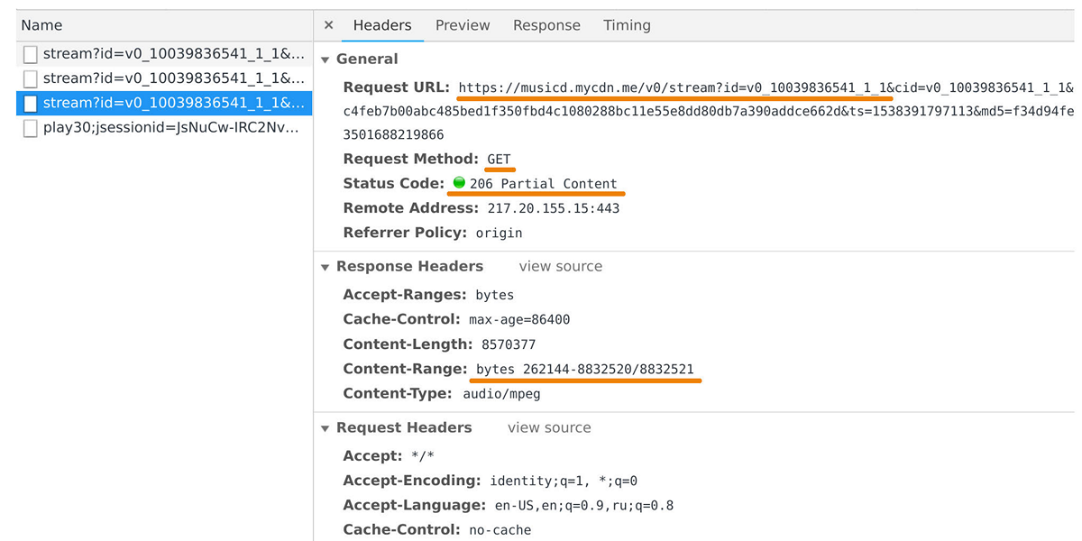



At peak load reaches 100 Gb / s through half a million connections. In fact, the music distributor is a cache front-end in front of our internal storage of tracks, which is based on One Blob Storage and One Cold Storage and contains petabytes of data.

Since I started talking about caching, let's look at the playback statistics. We see a pronounced TOP.



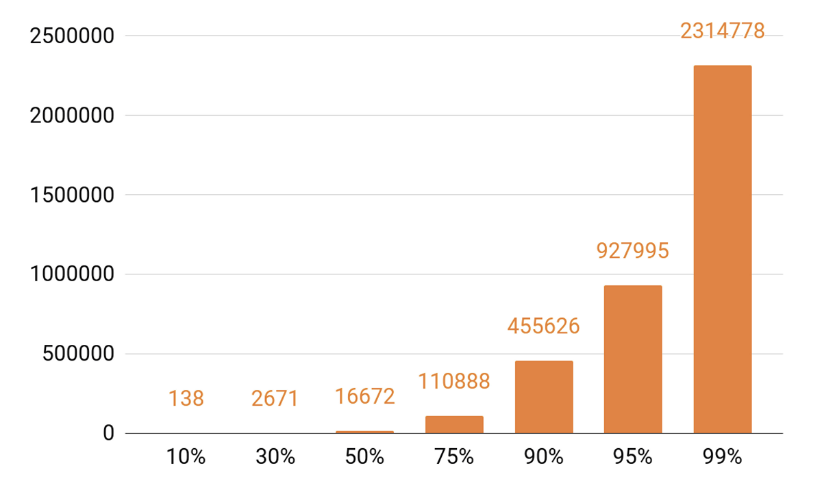
Approximately 140 tracks cover 10% of all auditions in a day. If we want our caching server to have a hit hit of at least 90%, then we need to put half a million tracks into it. 95% - almost a million tracks.

Distributor Requirements

What goals did we set when developing the next version of the distributor?

We wanted one node to hold 100 thousand connections. And these are slow client connections: a bunch of browsers and mobile applications through networks with varying speeds. At the same time, the service, like all our systems, must be scalable and fault-tolerant.

First of all, we need to scale the bandwidth of the cluster in order to keep up with the popularity of the service and be able to give more and more traffic. You also need to be able to scale the total capacity of the cluster cache, because cache hit directly depends on it and the share of requests that will go into the track repository.

Today it is necessary to be able to scale any distributed system horizontally, that is, add machines and data centers. But we wanted to implement and vertical scaling. Our typical modern server contains 56 cores, 0.5-1 TB of RAM, a 10 or 40 Gbps network interface and a dozen SSD disks.

Speaking of horizontal scalability, an interesting effect arises: when you have thousands of servers and tens of thousands of disks, something constantly breaks. Disc failure is a routine, we change them for 20-30 pieces a week. And server failures do not surprise anyone, 2-3 machines per day are replaced. We had to face data center failures, for example, in 2018 there were three such failures, and this is probably not the last time.

Why am I all this? When we design any systems, we know that they will break sooner or later. Therefore, we always carefully study the failure scenarios of all system components. The main way to deal with failures is to backup using data replication: several copies of data are stored on different nodes.

We also reserve network bandwidth. This is important, because if a component of the system fails, the load on the other components should not be allowed to collapse the system.

Balancing

First you need to learn how to balance user requests between data centers, and do it automatically. This is in case you need to conduct network work, or if the data center has failed. But balancing is also needed inside the data centers. Moreover, we want to distribute requests between nodes not randomly, but with weights. For example, when we post a new version of the service and we want to introduce a new node smoothly into the rotation. Weights also help a lot with load testing: we increase the weight and get much more workload on the node to understand the limits of its capabilities. And when the node fails under load, we quickly zero the weight and remove it from the rotation, using the mechanisms of balancing.

How does the query path from the user to the node, which will return the data, taking into account balancing?



The user logs in via the website or mobile application and receives the track URL:

musicd.mycdn.me/v0/stream?id=...

To get the IP address from the host name in the URL, the client contacts our GSLB DNS, which knows about all our data centers and CDN sites. GSLB DNS gives the client the IP address of the balancer of one of the data centers, and the client establishes a connection with it. The balancer knows about all the nodes inside the data centers and their weight. He on behalf of the user establishes a connection with one of the nodes. We use L4 balancers based on NFWare . The node gives the user data directly, bypassing the balancer. In services like a distributor, outgoing traffic significantly exceeds incoming traffic.

If a data center failure occurs, GSLB DNS detects this and promptly takes it out of rotation: it stops giving users the IP address of the balancer of this data center. If a node fails in the data center, then its weight is reset, and the balancer inside the data center stops sending requests to it.

Now consider the balancing of tracks on the nodes inside the data center. We will consider data centers as independent autonomous units, each of them will live and work, even if all the others died. Tracks need to be balanced on the machines evenly, so that there is no load imbalance, and replicate them to different nodes. If one node fails, the load should be distributed equally among the rest.

This problem can be solved in different ways . We stopped atconsistent hashing . The entire possible range of track identifier hashes is wrapped in a ring, and then each track is mapped to a point on this ring. Then we more or less evenly distribute the ring ranges between the nodes in the cluster. The nodes that will store the track are selected by hashing the tracks to a point on the ring and moving clockwise.



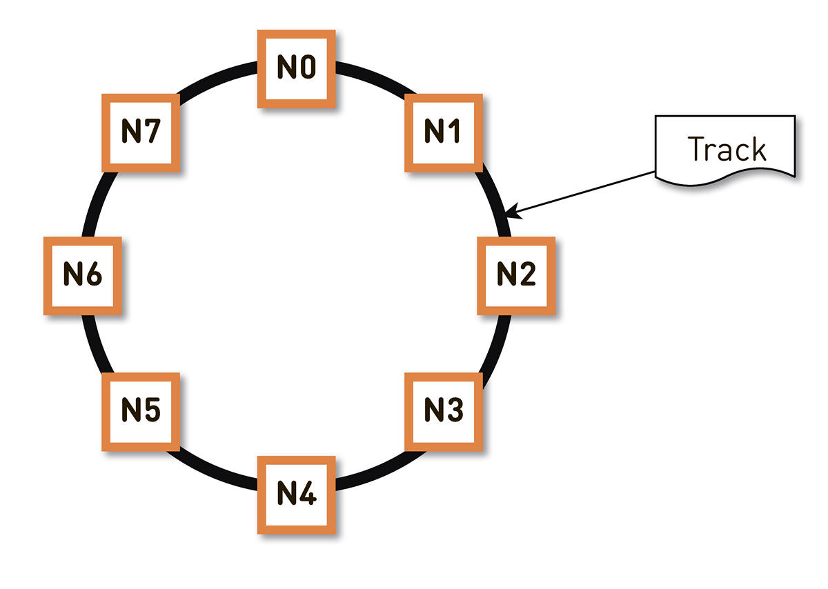
But such a scheme has a drawback: in the event of a failure of the N2 node, for example, its entire load will fall on the next cue along the ring - N3. And if it does not have a double performance margin - and this is not economically justified - then, most likely, the second node will also have to be bad. N3 with a high degree of probability will develop, the load will transfer to N4 and so on - a cascade failure will occur along the entire ring.

This problem can be solved by increasing the number of replicas, but then the total useful capacity of the cluster in the ring decreases. Therefore, we do otherwise. With the same number of nodes the ring is divided into a much larger number of ranges that are randomly scattered around the ring. Replicas for the track are selected by the above algorithm.



In the example above, each node is responsible for two ranges. If one of the nodes fails, its entire load will fall not on the next node around the ring, but will be distributed between two other nodes of the cluster.

The ring is calculated on the basis of a small set of parameters algorithmically and deterministically at each node. That is, we do not store it in some kind of config. We have more than one hundred thousand of these ranges in production, and in the event of a failure of any node, the load is distributed absolutely evenly among all other live nodes.

How does track output to a user in a consistent hashing system look like?

The user through the L4-balancer falls on a random node. The choice of the node is random, because the balancer knows nothing about the topology. But then every replica in the cluster knows about it. The node that receives the request determines whether it is a replica for the requested track. If not, it switches to proxy mode from one of the replicas, establishes a connection with it, and it searches for data in its local storage. If the track is not there, the replica pulls it out of the track repository, saves it to the local repository and gives the proxy, which forwards the data to the user.



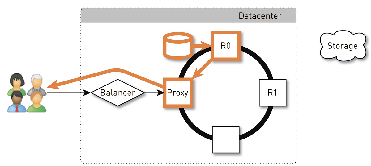
If the disk in the replica fails, the data from the storage will be transferred to the user directly. And if the replica fails, then the proxy knows about all the other replicas for this track, it will establish a connection with another live replica and receive data from it. So we guarantee that if a user has requested a track and at least one replica is alive, he will receive an answer.

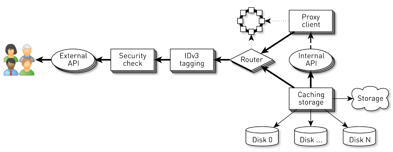
How does the node

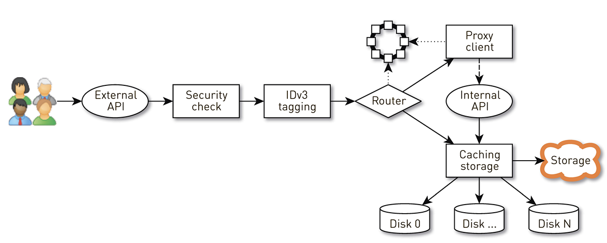
A node is a pipeline from a set of stages through which a user request passes. First, the request goes to the external API (we give everything via HTTPS). Further validation of the request is performed - signatures are checked. Then IDv3 tags are constructed, if necessary, for example, when purchasing a track. The request goes to the routing stage, where, based on the cluster topology, it is determined how the data will be given: either the current node is a replica for this track, or we will be proxying from another node. In the second case, the node through the proxy client establishes a connection to the replica via the internal HTTP API without checking signatures. The replica searches for data in the local storage, if it finds a track, it returns it from its disk; and if it does not find it, it pulls up tracks from the repository, caches and gives them away.

Load on node

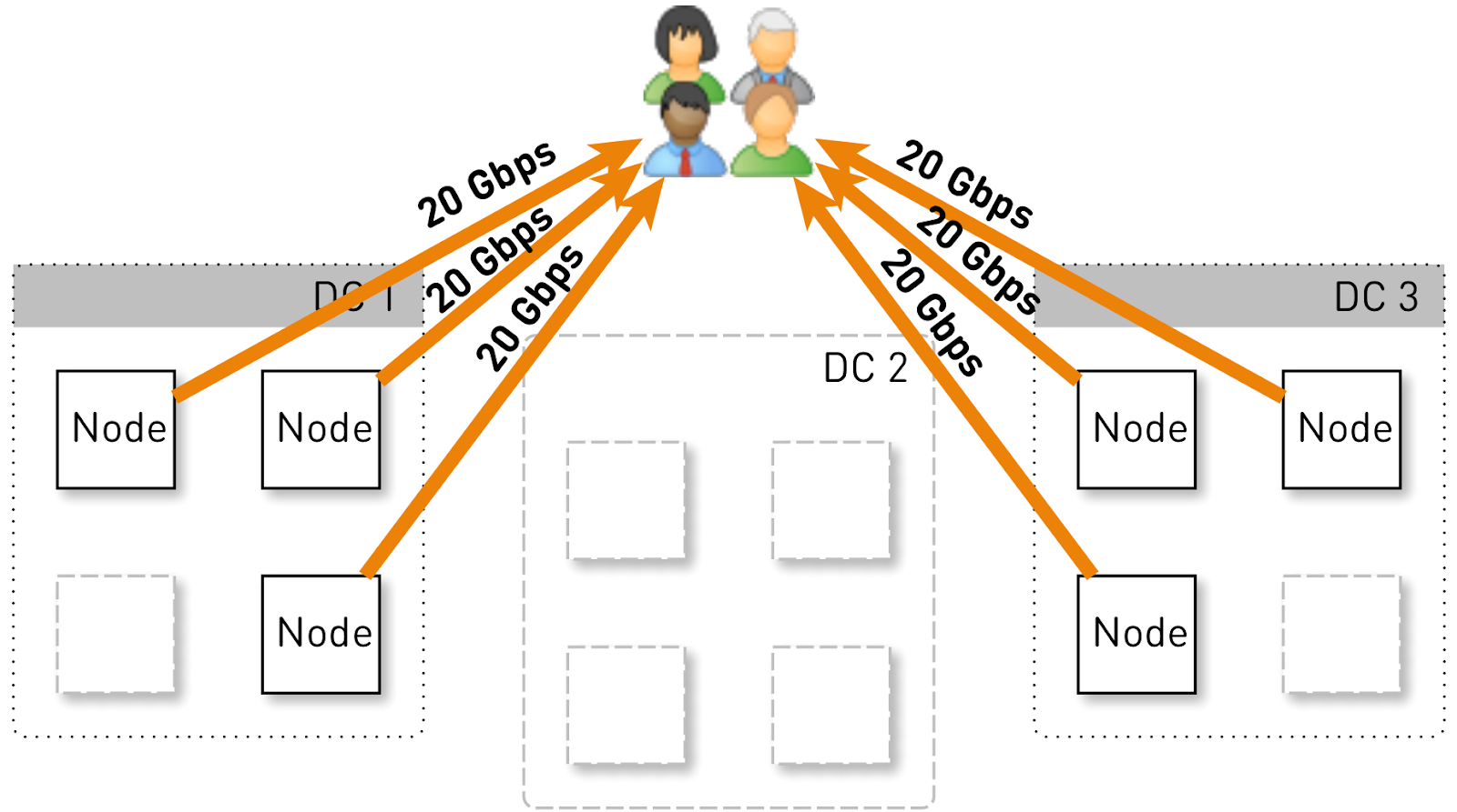
Let us estimate what load one node should hold in such a configuration. Suppose we have three data centers of four nodes.



The entire service should serve 120 Gbit / s, that is, 40 Gbit / s per data center. For example, networkers made maneuvers or an accident occurred, and two data centers DC1 and DC3 remained. Now each of them should give 60 Gbit / s. But here the developers wanted to roll out some kind of update, 3 live nodes remained in each data center and each of them should give 20 Gbit / s.



But initially there were 4 nodes in each data center. And if we store two replicas in the data center, then with a probability of 50% the node that received the request will not be a replica for the requested track and will begin to proxy the data. That is, half of the traffic inside the data center is proxied.



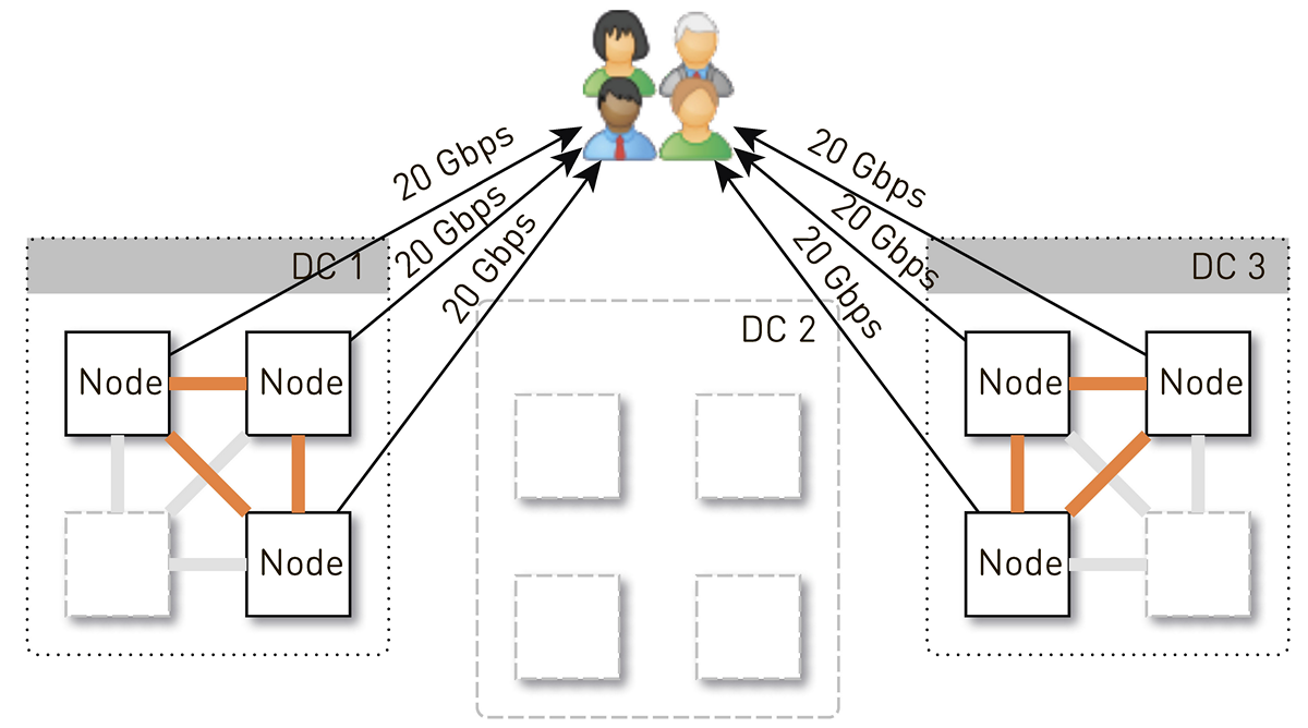
So, one node should give users 20 Gbit / s. Of these, 10 Gbps it pulls from its neighbors in the data center. But the scheme is symmetrical: the same 10 Gbit / s node gives its neighbors in the data center. It turns out that 30 Gbps comes from the node, of which 20 Gbps should serve itself, since it is a replica of the requested data. And the data will go either from the disks or from the RAM, where about 50 thousand "hot" tracks fit. Taking into account our statistics of playback, this allows removing 60-70% of the load from the disks, and about 8 Gbit / s will remain. This thread is quite capable of giving a dozen SSD.

Data storage on node

If each track is put in a separate file, then the overhead of managing these files will be huge. Even restarting the node and scanning the data on the disks will take minutes, if not tens of minutes.

There are less obvious limitations in this scheme. For example, you can load tracks only from the very beginning. And if the user requested playback from the middle and a cache miss occurred, then we will not be able to give a single byte until we load the data to the desired location from the track repository. Moreover, we can also store the tracks only as a whole, even if it is a gigantic audiobook, which is already abandoned in the third minute. It will lay like a dead weight on the disk, waste expensive space and reduce the cache hit of this node.

Therefore, we do it in a completely different way: we split up the tracks into blocks of 256 KB each, because this correlates with the size of the block in the SSD, and we are already operating with these blocks. 4 million blocks fit on a 1 TB disk. Each disk in the node is an independent storage, and all blocks of each track are distributed across all disks.

We did not immediately come to such a scheme, at first all the blocks of one track lay on one disc. But this led to strong load imbalances between the disks, since if one of the disks had hit a popular track, all requests for its data would fall on one disk. To avoid this, we distributed the blocks of each track across all discs, equalizing the load.

In addition, do not forget that we have a lot of RAM, but we decided not to do the samopisny cache, since we have a wonderful page cache in Linux.

How to store blocks on disks?

First, we decided to create one giant XFS file the size of a disk and place all the blocks in it. Then came the idea to work directly with the block device. We implemented both options, compared them and it turned out that when working directly with a block device, the recording is 1.5 times faster, the response time is 2-3 times lower, the overall system load is 2 times lower.

Index

But it is not enough to be able to store blocks, it is necessary to maintain an index from blocks of music tracks to blocks on a disk.



It turned out quite compact, one index record takes up only 29 bytes. For a storage size of 10 TB, the index takes a little more than 1 GB.

There is an interesting point. Each such record has to keep the total size of the entire track. This is a classic example of denormalization. The reason is that, according to the specification in the HTTP range response, we must return the total size of the resource, as well as form the Content-length header. If it were not for this, then everything would have been even more compact.

To the index, we formulated a number of requirements: to work quickly (preferably stored in RAM), so that it was compact and did not take up space from page cache. Another index must be persistent. If we lose it, we will lose information about where in the disk which track is stored, which is equivalent to cleaning the disks. And in general, it would be desirable that the old blocks, which have not been addressed for a long time, were somehow supplanted, freeing up space for more popular tracks. We chose the LRU crowding policy : the blocks are crowded out once a minute, we keep 1% of the blocks free. Of course, the index structure must be thread-safe, because we have 100 thousand connections per node. All these conditions are ideally satisfied SharedMemoryFixedMapfrom our open source library one-nio .

We put the index on tmpfs, it works quickly, but there is a nuance. When the machine restarts, everything is lost tmpfs, including the index. In addition, if due to любимого sun.misc.Unsafeour process collapsed, it is unclear in what condition the index remained. Therefore, we make an impression of it once an hour. But this is not enough: once we use block crowding, we have to maintain WAL , in which we write information about the crowded blocks. The block entries in the casts and the WAL need to be somehow streamlined during restoration. For this we use block generation. It plays the role of a global transaction counter and is incremented every time the index changes. Let's look at an example of how this works.

Take an index with three entries: two blocks of track # 1 and one block of track # 2.



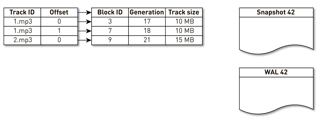
The stream of creation of impressions is awakened and it is iterated on this index: the first and second tuples fall into the impression. Then the displacement stream addresses the index, realizes that the seventh block has not been addressed for a long time, and decides to use it for something else. The process displaces the block and writes an entry to WAL. He gets to block 9, sees that he, too, has not been contacted for a long time, and also marks him as repressed. Here the user accesses the system and a cache miss occurs - a track is requested that we don’t have. We save the block of this track to our storage, overwriting block 9. In this case, the generation is incremented and becomes equal to 22. Next, the process of creating an impression is activated, which has not completed its work, reaches the last record and writes it to the impression. As a result, we have two live recordings in the index, a cast and a WAL.



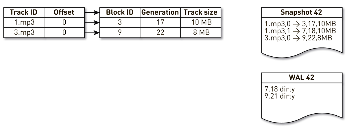
When the current node falls, it will restore the initial state of the index as follows. First, we scan the WAL and build a map of dirty blocks. The map stores the mapping from the block number to the generation when this block was preempted.



After that, we start to iterate over the image, using the map as a filter. We look at the first record of the cast, it concerns the block №3. He is not mentioned among the dirty, so he is alive and falls into the index. We get to block number 7 with the eighteenth generation, but the map of dirty blocks tells us that just in the 18th generation, the block was ousted. Therefore, it does not enter the index. We reach the last entry, which describes the contents of block 9 with 22 generation. This block is mentioned in the map of dirty blocks, but it was ousted earlier. This means that it is reused for new data and is indexed. The goal is achieved.

Optimization

But that's not all, we go down deeper.

Let's start with page cache. We were counting on it initially, but when we started to conduct load testing of the first version, it turned out that page cache hit rate does not reach 20%. We assumed that the problem is in read ahead: we do not store files, but blocks, while serving a bunch of connections, and in such a configuration it is efficient to work with the disk randomly. We almost never read anything consistently. Fortunately, there is a call in Linux posix_fadvisethat allows you to tell the kernel how we are going to work with the file descriptor - in particular, we can say that we don’t need to read ahead by passing the flag POSIX_FADV_RANDOM. This system call is available through one-nio. In operation, our cache hit is 70-80%. The number of physical reads from disks decreased by more than 2 times, the HTTP response delay decreased by 20%.

Let's move on. The service has a rather large size heap. To make life easier for the processor's TLB caches, we decided to enable Huge Pages for our Java process. As a result, we received a noticeable profit for the time of garbage collection (GC Time / Safepoint Total Time is 20-30% lower), the load on the cores became more uniform, but we did not notice any effect on the HTTP latency charts.

Incident

Soon after the launch of the service, a single (so far) incident occurred.

One evening after the end of the working day, complaints about playing music fell down in support. Users wrote that they include their favorite track, but every few seconds they hear incomprehensible music from other times and peoples, and the player tells them that this is their favorite track. Pretty quickly narrowed down the search to one car, which gave something strange. The logs found that it was recently restarted. If to simplify, then we had two disks and indexes that described the contents of the blocks. One index says that the fourth block of the Daft Punk track lies in block 2 of the sdc disk, and the zero block of the Stas Mikhailov track lies in the zero block of the sdd disk.



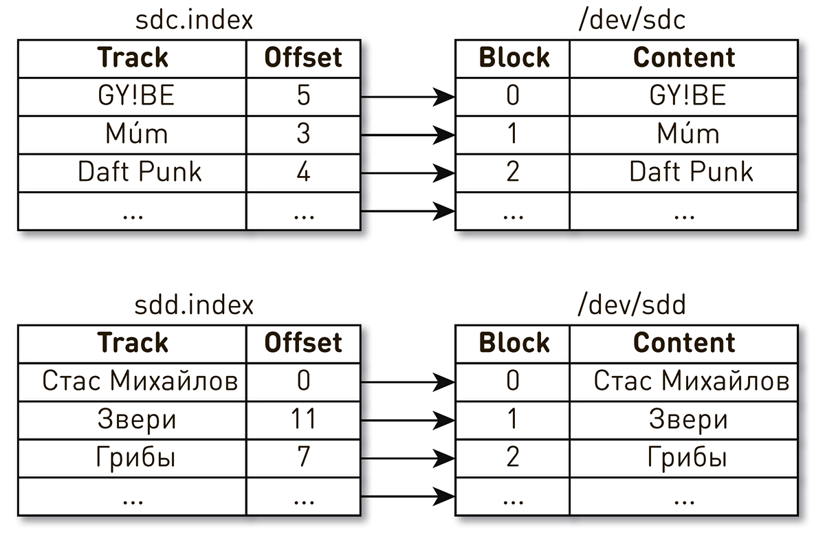
It turned out that after rebooting the machine, the drive names changed places with all the ensuing consequences. This problem in Linux is well known : if there are several disk controllers in the server, then the order of naming the disks is not guaranteed.



The fix turned out to be simple. There are several different types of persistent IDs for disks. We use WWN based on the serial numbers of the disks and identify with their help indexes, snapshots and WAL. This does not exclude the mixing of the disks, but no matter how they are mixed, the map indexes on the disk will not be disturbed and we will always give the correct data.

Incident Analysis

The analysis of problems in such distributed systems is difficult, because a user request goes through many stages and crosses the borders of the nodes. In the case of CDN, everything becomes even more complicated, because for CDN an upstream is a home data center. There are quite a few such hopes. Moreover, the system serves hundreds of thousands of user connections. It is quite difficult to understand at what stage the problem arises with the processing of a particular user's request.

We simplify our life so. At the entrance to the system, we mark all requests with a tag, by analogy with Open Tracing and Zipkin.. The tag includes the user ID, the request and the requested track. This tag inside the pipeline is transmitted with all the data and requests related to the current connection, and between nodes is transmitted as an HTTP header and is restored by the receiving party. When we need to deal with the problem, we turn on debugging, log the tag, find all the records related to a particular user or track, aggregate and find out how the request was processed all the way through the cluster.

Sending data

Consider a typical scheme for sending data from disk to socket. It seems nothing complicated: select the buffer, read from the disk to the buffer, send the buffer to the socket.

ByteBuffer buffer = ByteBuffer.allocate(size);
int count = fileChannel.read(buffer, position);
if (count <= 0) {
   // ...
}
buffer.flip();
socketChannel.write(buffer);

One of the problems with this approach is that two hidden data copies are hidden here:

• when reading from a file using FileChannel.read(), copying from the kernel space to the user space takes place;
• and when we send data from the buffer to the socket using SocketChannel.write(), copying from user space to the kernel space takes place.

Fortunately, there is a call in Linux sendfile()that allows you to ask the kernel to send data from a file to a socket from a certain offset directly, bypassing copying to user space. And of course, this call is available through one-nio . We on load tests started user traffic to one node and forced to proxy from a neighboring node, which gave data only through sendfile()- the processor load at 10 Gbit / s when used sendfile()was close to 0.

But in the case of user-space SSL sockets use sendfile()and we have nothing left but to send data from the file through the buffer. And here we are waiting for another surprise. If you delve into the source SocketChanneland FileChannel, or use Async Profilerand poprofilirovat system in the process of return data in a manner that sooner or later you get to the class sun.nio.ch.IOUtilto which boil down all calls read(), and write()on these channels. There is hidden such a code.

ByteBuffer bb = Util.getTemporaryDirectBuffer(dst.remaining());
try {
    int n = readIntoNativeBuffer(fd, bb, position, nd);
    bb.flip();
    if (n > 0)
        dst.put(bb);
    return n;
} finally {
    Util.offerFirstTemporaryDirectBuffer(bb);
}

This is a pool of native buffers. When you read from a file in heap ByteBuffer, the standard library first takes a buffer from this pool, reads data into it, then copies it to your heap ByteBuffer, and returns the native buffer back to the pool. When writing to a socket, the same thing happens.

Controversial scheme. Here one-nio comes to the rescue again . We create an allocator MallocMT- in fact, this is a pool of memory. If we have SSL and we have to send data through a buffer, then we allocate the buffer outside of the Java heap, wrap it in ByteBuffer, read it without copying it from FileChannelthis buffer, and write to the socket. And then we return the buffer to the allocator.

final Allocator allocator = new MallocMT(size, concurrency);
intwrite(Socket socket){
    if (socket.getSslContext() != null) {
        long address = allocator.malloc(size);
        ByteBuffer buf = DirectMemory.wrap(address, size);
        int available = channel.read(buf, offset);
        socket.writeRaw(address, available, flags);

100,000 connections per node

But the success of the system is not guaranteed by the reasonableness of implementation at the lower levels. There is another problem here. The pipeline on each node serves up to 100 thousand simultaneous connections. How to organize calculations in such a system?

The first thing that comes to mind is to create a flow of execution for each client or connection and in it we perform the stages of the pipeline one by one. If necessary, block, then go ahead. But with such a scheme, the costs of context switches and flow stacks will be excessive, since we are talking about the distributor and there are a lot of flows. Therefore, we went a different way.



For each connection, a logical pipeline is created which consists of stages interacting with each other asynchronously. Each stage has its turn, which stores incoming requests. For the execution of the stages small common thread pools are used. If we need to process the message from the request queue, we take the stream from the pool, process the message, and return the stream to the pool. With such a scheme, data is pushed from storage to the client.

But such a scheme is not without flaws. Backends work much faster than user connections. When data passes through a pipeline, it accumulates at the slowest stage, i.e. at the stage of writing blocks to the client connection socket. Sooner or later it will lead to the collapse of the system. If you try to limit the queues at these stages, then everything will instantly stall, because the pipelines in the chain to the user's socket will be blocked. And since they use shared thread pools, they will block all threads in them. Need back pressure.

For this, we used jet streams.. The essence of the approach is that the subscriber controls the speed of data arrival from the publisher using demand. Demand means how much more data is ready to process a subscriber along with previous demand, which it has already signaled. Publisher has the right to send data, but only not exceeding the total accumulated demand at the moment minus the data already sent.

Thus, the system dynamically switches between push and pull modes. In push mode, a subscriber is faster than publisher, that is, publisher always has unsatisfied demand from a subscriber, but there is no data. As soon as the data appears, he immediately sends them to the subscriber. Pull mode occurs when publisher is faster than subscriber. That is, publisher would be happy to send data, only demand is zero. As soon as the subscriber reports that he is ready to process a little more, the publisher will immediately send him a portion of the data as part of the demand.

Our conveyor turns into jet stream. Each stage turns into a publisher for the previous stage and a subscriber for the next.

The interface of jet streams looks extremely simple. Publisherallows you to signSubscriber, and he should only implement four handlers:

interfacePublisher<T> {
    voidsubscribe(Subscriber<? super T> s);
}
interfaceSubscriber<T> {
    voidonSubscribe(Subscription s);
    voidonNext(T t);
    voidonError(Throwable t);
    voidonComplete();
}
interfaceSubscription{
    voidrequest(long n);
    voidcancel();
}

Subscriptionallows you to signal demand and cancel a subscription. There is simply no place.

As a data element, we are not passing arrays of bytes, but rather an abstraction like chunk. We do this in order not to delay data in heap, if possible. Chunk is a link to data with a very limited interface that only allows you to read data into ByteBuffer, write to a socket or to a file.

interfaceChunk{
    intread(ByteBuffer dst);
    intwrite(Socket socket);
    voidwrite(FileChannel channel, long offset);
}

There are many implementations of chunks:

• The most popular, which is used in the case of cache hit and when transferring data from the disk, is the implementation on top RandomAccessFile. The chunk contains only a link to the file, an offset in that file and the size of the data. It goes through the entire pipeline, reaches the socket of the user connection and turns into a call there sendfile(). That is, memory is not consumed at all.
• In the case of cache miss, a different implementation is used: we extract the track from our storage block by block and save it to disk. The chunk contains a reference to the socket, - in fact, the client connection in the track repository, - the position in the stream and the size of the data.
• Finally, in the case of proxying, it is still necessary to place the received block in the heap. Here the chunk acts as a wrapper around ByteBuffer.

Despite the simplicity of this API, according to the specification it must be thread safe, and most methods must be non-blocking. We chose a path in the spirit of the Typed Actor Model, inspired by examples from the official repository of jet streams . To make the method calls non-blocking, when we call the method, we take all the parameters, wrap the message, put it in the queue for execution, and return control. Messages from the queue are processed strictly sequentially.


We have a completely non-blocking implementation. Code simple and consistent, without volatile, Atomic*, contention, and others. There are only 200 threads in our entire system for servicing 100,000 connections.

Eventually

In production, we have 12 machines, while there is more than a double margin on throughput. Each machine normally gives up to 10 Gbps through hundreds of thousands of connections. We have provided scalability and fault tolerance. Everything is written in Java and one-nio .



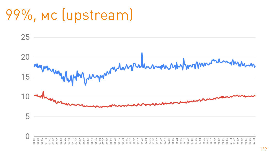
This is a graph up to the first byte given to the user by the server. 99-percentile is less than 20 ms. The blue graph is the return to the user of the HTTPS data. The red graph is the return of data from the replica to the proxy via sendfile()HTTP.

In fact, cache hit in production 97%, so the charts describe the latency of our track repository, from which we pull up data in the case of cache misses, which is also a good thing, given the petabytes of data.



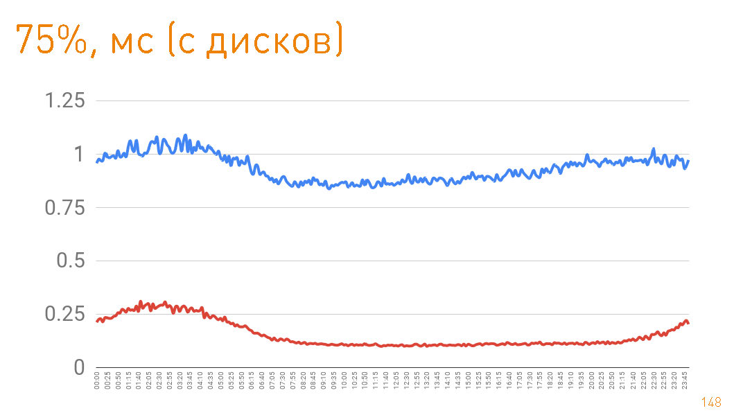
If you look at the 75th percentile when returning from disks, then the first byte flies to the user after 1 ms. Replicas inside the cluster communicate with even greater speed - they are responsible for 300 µs. Those. 0.7 ms is the cost of proxying.

In this article, we wanted to demonstrate how we build scalable high-load systems that have both high speed and excellent fault tolerance. We hope we did it.