Crib for artificial intelligence - throw away too much, teach the main thing. Technique processing training sequences
This is the second article on the analysis and study of materials competition for the search for ships at sea. But now we will study the properties of training sequences. Let's try to find in the source data extra information, redundancy and remove it.
This article, too, is simply the result of curiosity and idle interest, nothing of it is found in practice, and for practical tasks there is almost nothing to copy-paste. This is a small study of the properties of the training sequence - the author's reasoning and the code are set forth; everything can be checked / supplemented / modified by oneself.
Recently ended kaggle competition for finding ships at sea. Airbus offered to analyze satellite images of the sea, both with and without vessels. A total of 192555 768x768x3 pictures is 340 720 680 960 bytes if uint8 and this is a huge amount of information and there is a vague suspicion that not all the pictures are needed for network training and in this amount of information repetitions and redundancy are obvious. When training a network, it is common practice to separate some of the data and not use it in training, but use it to test the quality of training. And if the same section of the sea hit two different snapshots and one snapshot got into the training sequence, and the other into the test sequence, then the check will lose its meaning and the network will be retrained, we will not check the network property to summarize the information, because the data is the same. The struggle against this phenomenon has taken away a lot of time and effort of the GPU participants. As usual, the winners and runners-ups are not in a hurry to show their fans the secrets of mastery and lay out the code and there is no way to study and learn it, so let's do the theory.
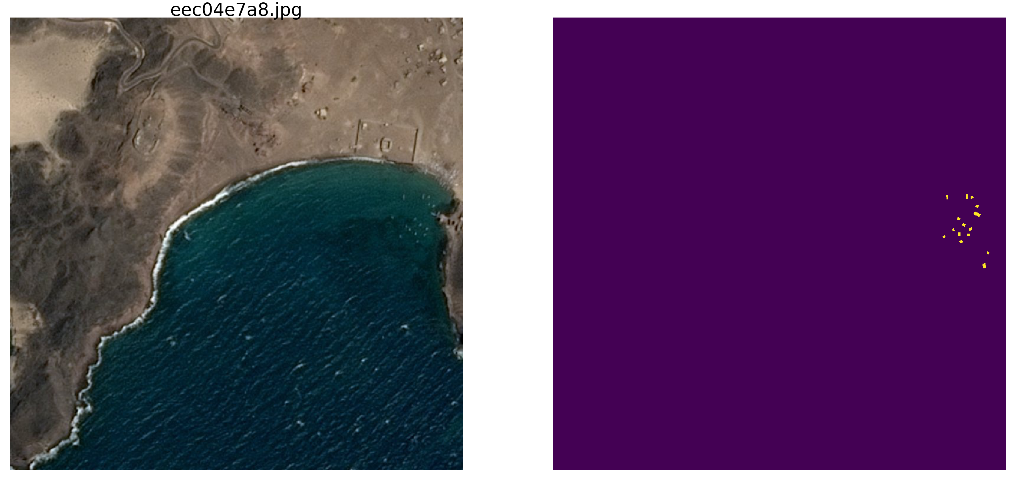
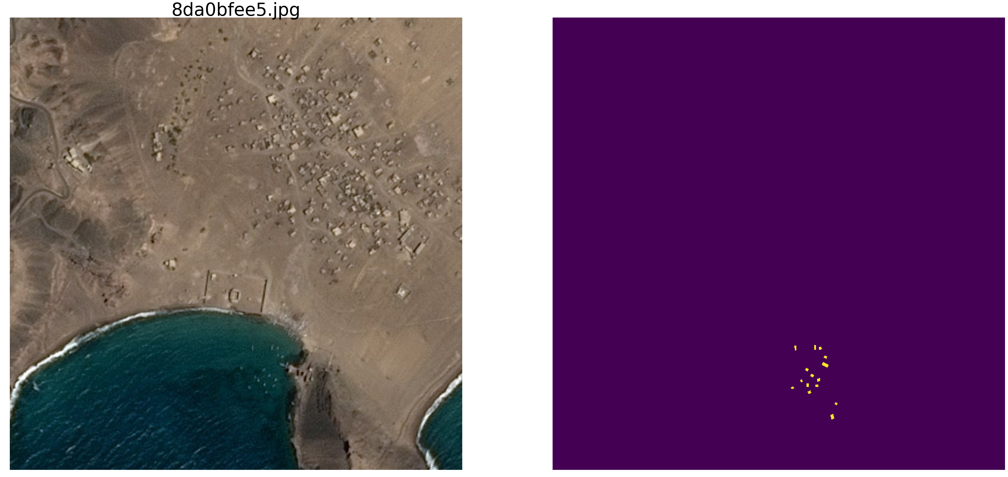
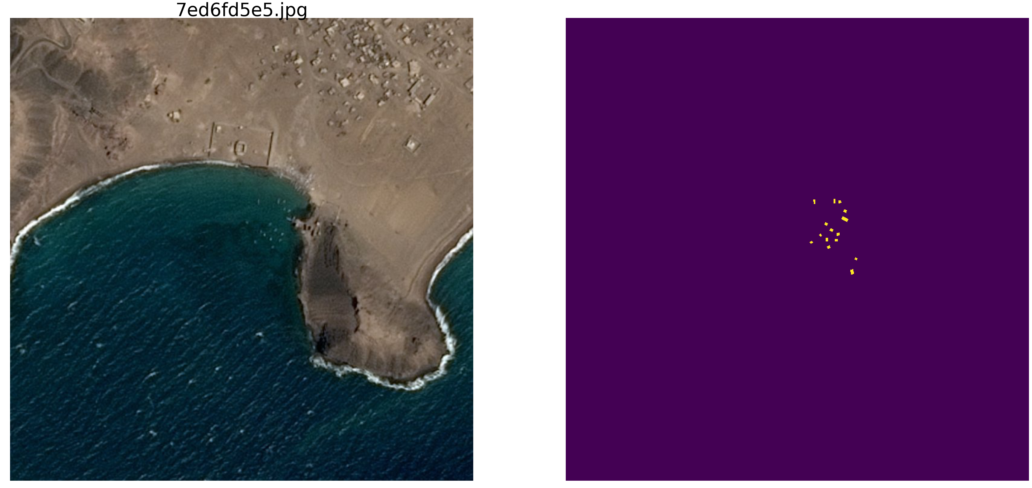
The simplest visual verification showed that there was indeed too much data, the same section of the sea got into different pictures, look at the examples.
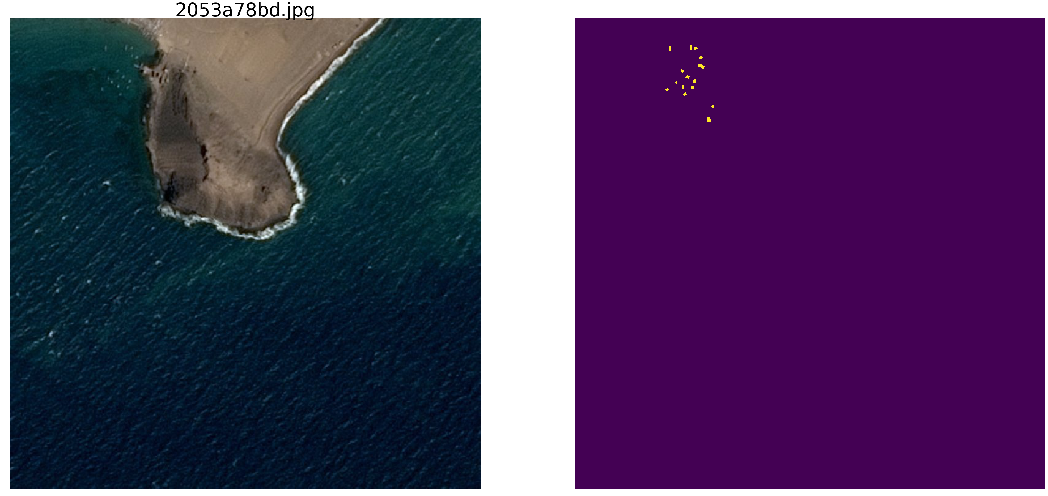
For this reason, the real data is not interesting for us, there are a lot of parasitic dependencies, unnecessary links to us, bad markup and other shortcomings.
In the first article, we looked at pictures with ellipses and noise, so let's continue to study them. The advantage of this approach is that if you find any attractive feature of a network trained in an arbitrary set of pictures, then it is not clear whether this is a property of the network or a property of the training set. The statistical parameters of sequences taken from the real world are unknown. Recently Grandmaster Paleskov Pavel paske57 toldhow sometimes it is easy to win a competition on segmentation / classification of pictures, if you delve into the data yourself, for example, to look at the metadata of photos. And there are no guarantees that there are no dependencies in real data of such involuntarily left. Therefore, we take to study the properties of the network pictures with ellipses and rectangles, and the place and color and other parameters are determined using a computer’s random number generator (who has a pseudo-random generator, who has a generator based on other non-digital algorithms and physical properties of a substance, But this will not be discussed in this article).
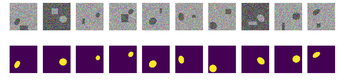
So, take the sea np.random.sample () * 0.75, we do not need waves, wind, shores and other hidden patterns and faces. We will also color the ships / ellipses in the same color and in order to distinguish the sea from the ship and interference we add 0.25 to the sea or the ship / disturbance, and they will all be of the same shape - ellipses of different size and orientation. Interference will also be only rectangles of the same color as the ellipse - this is important, information and interference of the same color against the background of noise. We make only a small change in the coloring and we will run np.random.sample () for each image and for each ellipse / rectangle, i.e. neither the background nor the color of the ellipse / rectangle is repeated. Further in the text there is a code of the program for creating pictures / masks and an example of ten randomly selected pairs.
Take a very common version of the network (you can take your favorite network) and try to identify and show the redundancy of a large training sequence, get at least some qualitative and quantitative characteristics of redundancy. Those. The author believes that many gigabytes of training sequences are redundant substantially, there are a lot of unnecessary pictures, there is no need to load dozens of GPUs and do unnecessary calculations. The data redundancy is manifested not only and not so much in that the identical parts are displayed in different pictures, but also in the redundancy of information in these data. Data may be redundant, even if it does not repeat exactly. Please note that this is not a strict definition of information and its sufficiency or redundancy. We just want to find out how much you can cut the train, which pictures can be thrown out of the training sequence and how many pictures are enough for acceptable (let us specify the accuracy in the program) training. This is a specific program, a specific dataset, and it is possible that on ellipses with triangles, as a hindrance, nothing will work the same way as on ellipses with rectangles (my hypothesis: that everything will be the same and the same. But now we don’t check , analysis is not carried out and we do not prove theorems).
So, given:
Idea for verification:
Let's start, choose 10,000 pairs and consider them carefully. We will squeeze out all the water from this training sequence, all the unnecessary bits, and use and use the whole dry residue.
You can now test your intuition and assume how many pairs of 10,000 are enough to train and predict another, but also created, sequence of 10,000 pairs with an accuracy greater than 0.98. Write down on a piece of paper, after compare.
For practical application, please note that both the sea and ships with noises are artificially selected, this is np.random.sample () .
We will use the metric from the first article . Let me remind readers that we will predict the pixel mask - this is the "sea" or "ship" and evaluate the truth or falsity of the prediction. Those. the following four options are possible - we correctly predicted that a pixel is a “sea”, correctly predicted that a pixel is a “ship” or made a mistake in predicting a “sea” or “ship”. And so on all the pictures and all the pixels we estimate the number of all four options and calculate the result - this will be the result of the network. And the fewer erroneous predictions and the more true, the more accurate the result and the better the operation of the network.
And for research we will take the option of a well-studied U-net, this is an excellent network for image segmentation. The not quite classic version of U-net was chosen, but the idea is the same; the network performs a very simple operation with pictures — step by step reduces the dimension of the picture with some transformations and then tries to restore the mask from the compressed image. Those. in our case, the dimension of the image is reduced to 16x16 and then we try to restore the mask using data from all previous compression layers.
We examine the network as a “black box”, we will not look at what is happening with the network inside, how weights change and how gradients are selected - this is a topic for another study.
The function of generating pairs of image / mask. On the color picture 128x128 filled with random noise with a randomly selected from two ranges, or 0.0 ... 0.75 or 0.25.1.0. Randomly in the picture we place a randomly oriented ellipse and place a rectangle in the same place. We check that they do not intersect and move the rectangle to the side if necessary. Each time we re-consider the values of the coloring of the sea / ship. For simplicity, we will place the mask with a picture in one array, as the fourth color, i.e. Red.Green.Blue.Mask is easier.
Create a training sequence of pairs, see random 10.
The first step of our experiment is simple, we are trying to train the network to predict only 11 first pictures.
We selected the first 11 from the initial sequence and trained the network on them. Now it doesn’t matter whether the network memorizes these particular pictures or generalizes, the main thing is that it can recognize these 11 pictures as we need. Depending on the chosen dataset and accuracy, network training can last for a long, very long time. But we have only a few iterations. I repeat that now it does not matter to us how or what the network has learned or learned, the main thing is that it has achieved the established prediction accuracy.
We will take new picture / mask pairs from the constructed sequence and will try to predict them with a network trained on the already selected sequence. At the beginning it is only 11 pairs of picture / mask and the network is trained, perhaps not very well. If a new mask is predicted for a picture with acceptable accuracy, then we throw out this pair, it does not contain new information for the network, it already knows and can calculate a mask from this picture. If the prediction accuracy is insufficient, then this masked image is added to our sequence and we begin to train the network to achieve an acceptable accuracy result on the selected sequence. Those. This picture contains new information and we add it to our training sequence and extract the information contained in it by training.
Here accuracy is used in the sense of “accuracy”, and not as the standard metric keras, and the subroutine “my_iou_metric” is used to calculate the accuracy. It is very interesting to observe the accuracy and the number of investigated and added pictures. At the beginning, almost all pairs of picture / mask network adds, and somewhere around 70 it starts to throw out already. Closer to 8000 throws almost all pairs.
Check visually random pairs selected by the network:
Nothing fancy or supernatural:
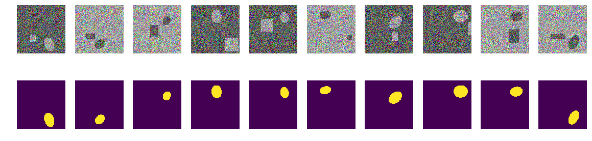
These are pairs chosen by the network at different stages of learning. When the network received a pair from this sequence as input, it could not compute the mask with the specified accuracy and this pair was included in the training sequence. But nothing special, ordinary pictures.
Check the quality of the network training program, make sure that the quality does not significantly depend on the order of the original sequence, for which we mix the original sequence of the picture / mask pairs, take the other 11 first ones and also, by the same method, train the network and cut off the excess.
The result is not significantly dependent on the order of the pairs of the original sequence. In the previous case, the network chose 271, now it’s 408, if you mix it up, the network can choose a different quantity. We will not check, the author believes that there will always be substantially less than 10,000. We will
verify the accuracy of network prediction on a new independent sequence.
So, we were able to squeeze out of less than three or four hundred, selected from 10,000 pairs, the prediction accuracy of 0.99278, we took all the pairs that contain at least some useful information and threw away the rest. We did not align the statistical parameters of the training sequence, add repeatability of information, etc. and did not use statistical methods at all. We take a picture that contains an unknown network yet information and squeeze everything out of it into a network weight. If the network meets at least one "mysterious" picture, then it will use it all in the business.
A total of 271 pairs of pictures / masks contain information for predicting 10,000 pairs with an accuracy of at least 0.8075 on each pair, that is, the total accuracy of the entire sequence is higher, but in each picture it is not less than 0.8075, we do not have pictures that we don’t we can predict and we know the lower bound of this prediction. (here, of course, the author has boasted, as without it, the article has neither verification of this statement, about 0.8075, nor proof, but most likely this is true)
To train a network, there is no need to load the GPU with everything that came to hand, you can pull out such a core of the train and train the network on it as the beginning of training. As you receive new images, you can manually mark up those that the network could not predict and add them to the core of the train, having retrained the network again, in order to squeeze out all the information from the new images. And there is no need to single out the validation sequence, we can assume that everything else except the one selected is a validation sequence.
Another mathematically not strict, but very important note. It is safe to say that each picture / mask pair contains “a lot” of information. Each pair contains “a lot” of information, although the majority of the picture / mask information pairs overlap or repeat. Each of the 271 picture / mask pairs contains information essential for prediction, and this pair cannot simply be thrown away.
Well, and a small note about the folds, many experts and kaggler-s divide the training sequence into folds and train them separately, combining the results obtained in a cunning way. In our case, it is also possible to divide into folds in the same way, if 271 pairs out of 10,000 are removed, then the remaining ones can also be used to create a new root sequence, which obviously gives a different, but comparable result. You can simply mix and take the other initial 11, as shown above.
The article provided the code and shows how to train U-net for image segmentation. This is a concrete example and the article intentionally does not contain any generalizations to other networks, to other sequences, there is no stern mathematics, everything is told and shown “on the fingers”. Just an example of how you can learn the network and at the same time achieve acceptable accuracy.
This article, too, is simply the result of curiosity and idle interest, nothing of it is found in practice, and for practical tasks there is almost nothing to copy-paste. This is a small study of the properties of the training sequence - the author's reasoning and the code are set forth; everything can be checked / supplemented / modified by oneself.
Recently ended kaggle competition for finding ships at sea. Airbus offered to analyze satellite images of the sea, both with and without vessels. A total of 192555 768x768x3 pictures is 340 720 680 960 bytes if uint8 and this is a huge amount of information and there is a vague suspicion that not all the pictures are needed for network training and in this amount of information repetitions and redundancy are obvious. When training a network, it is common practice to separate some of the data and not use it in training, but use it to test the quality of training. And if the same section of the sea hit two different snapshots and one snapshot got into the training sequence, and the other into the test sequence, then the check will lose its meaning and the network will be retrained, we will not check the network property to summarize the information, because the data is the same. The struggle against this phenomenon has taken away a lot of time and effort of the GPU participants. As usual, the winners and runners-ups are not in a hurry to show their fans the secrets of mastery and lay out the code and there is no way to study and learn it, so let's do the theory.
The simplest visual verification showed that there was indeed too much data, the same section of the sea got into different pictures, look at the examples.
For this reason, the real data is not interesting for us, there are a lot of parasitic dependencies, unnecessary links to us, bad markup and other shortcomings.
In the first article, we looked at pictures with ellipses and noise, so let's continue to study them. The advantage of this approach is that if you find any attractive feature of a network trained in an arbitrary set of pictures, then it is not clear whether this is a property of the network or a property of the training set. The statistical parameters of sequences taken from the real world are unknown. Recently Grandmaster Paleskov Pavel paske57 toldhow sometimes it is easy to win a competition on segmentation / classification of pictures, if you delve into the data yourself, for example, to look at the metadata of photos. And there are no guarantees that there are no dependencies in real data of such involuntarily left. Therefore, we take to study the properties of the network pictures with ellipses and rectangles, and the place and color and other parameters are determined using a computer’s random number generator (who has a pseudo-random generator, who has a generator based on other non-digital algorithms and physical properties of a substance, But this will not be discussed in this article).
So, take the sea np.random.sample () * 0.75, we do not need waves, wind, shores and other hidden patterns and faces. We will also color the ships / ellipses in the same color and in order to distinguish the sea from the ship and interference we add 0.25 to the sea or the ship / disturbance, and they will all be of the same shape - ellipses of different size and orientation. Interference will also be only rectangles of the same color as the ellipse - this is important, information and interference of the same color against the background of noise. We make only a small change in the coloring and we will run np.random.sample () for each image and for each ellipse / rectangle, i.e. neither the background nor the color of the ellipse / rectangle is repeated. Further in the text there is a code of the program for creating pictures / masks and an example of ten randomly selected pairs.
Take a very common version of the network (you can take your favorite network) and try to identify and show the redundancy of a large training sequence, get at least some qualitative and quantitative characteristics of redundancy. Those. The author believes that many gigabytes of training sequences are redundant substantially, there are a lot of unnecessary pictures, there is no need to load dozens of GPUs and do unnecessary calculations. The data redundancy is manifested not only and not so much in that the identical parts are displayed in different pictures, but also in the redundancy of information in these data. Data may be redundant, even if it does not repeat exactly. Please note that this is not a strict definition of information and its sufficiency or redundancy. We just want to find out how much you can cut the train, which pictures can be thrown out of the training sequence and how many pictures are enough for acceptable (let us specify the accuracy in the program) training. This is a specific program, a specific dataset, and it is possible that on ellipses with triangles, as a hindrance, nothing will work the same way as on ellipses with rectangles (my hypothesis: that everything will be the same and the same. But now we don’t check , analysis is not carried out and we do not prove theorems).
So, given:
- picture / mask pairs training sequence. We can generate any number of pairs of pictures / masks. I will immediately answer the question - why is the color and background random? I will answer simply, briefly, clearly and exhaustively, that I like it so much, an extra essence in the form of a border is not needed;
- the network is ordinary, ordinary U-net, slightly modified and widely used for segmentation.
Idea for verification:
- in the constructed sequence, as in real-life tasks, gigabytes of data are used. The author believes that the size of the training sequence is not so critical and the data should not necessarily be much, but they should contain “a lot” of information. This number, ten thousand pairs of pictures / masks, is not needed and the network will learn on a much smaller amount of data.
Let's start, choose 10,000 pairs and consider them carefully. We will squeeze out all the water from this training sequence, all the unnecessary bits, and use and use the whole dry residue.
You can now test your intuition and assume how many pairs of 10,000 are enough to train and predict another, but also created, sequence of 10,000 pairs with an accuracy greater than 0.98. Write down on a piece of paper, after compare.
For practical application, please note that both the sea and ships with noises are artificially selected, this is np.random.sample () .
Load the library, determine the size of the array of images
import numpy as np
import matplotlib.pyplot as plt
%matplotlib inline
import math
from tqdm import tqdm
from skimage.draw import ellipse, polygon
from keras import Model
from keras.optimizers import Adam
from keras.layers import Input,Conv2D,Conv2DTranspose,MaxPooling2D,concatenate
from keras.layers import BatchNormalization,Activation,Add,Dropout
from keras.losses import binary_crossentropy
from keras import backend as K
import tensorflow as tf
import keras as keras
w_size = 128
train_num = 10000
radius_min = 10
radius_max = 20
define loss and accuracy functions
defdice_coef(y_true, y_pred):
    y_true_f = K.flatten(y_true)
    y_pred = K.cast(y_pred, 'float32')
    y_pred_f = K.cast(K.greater(K.flatten(y_pred), 0.5), 'float32')
    intersection = y_true_f * y_pred_f
    score = 2. * K.sum(intersection) / (K.sum(y_true_f) + K.sum(y_pred_f))
    return score
defdice_loss(y_true, y_pred):
    smooth = 1.
    y_true_f = K.flatten(y_true)
    y_pred_f = K.flatten(y_pred)
    intersection = y_true_f * y_pred_f
    score = (2. * K.sum(intersection) + smooth) / (K.sum(y_true_f) + K.sum(y_pred_f) + smooth)
    return1. - score
defbce_dice_loss(y_true, y_pred):return binary_crossentropy(y_true, y_pred) + dice_loss(y_true, y_pred)
defget_iou_vector(A, B):# Numpy version
    batch_size = A.shape[0]
    metric = 0.0for batch in range(batch_size):
        t, p = A[batch], B[batch]
        true = np.sum(t)
        pred = np.sum(p)
        # deal with empty mask firstif true == 0:
            metric += (pred == 0)
            continue# non empty mask case.  Union is never empty # hence it is safe to divide by its number of pixels
        intersection = np.sum(t * p)
        union = true + pred - intersection
        iou = intersection / union
        # iou metrric is a stepwise approximation of the real iou over 0.5
        iou = np.floor(max(0, (iou - 0.45)*20)) / 10
        metric += iou
    # teake the average over all images in batch
    metric /= batch_size
    return metric
defmy_iou_metric(label, pred):# Tensorflow versionreturn tf.py_func(get_iou_vector, [label, pred > 0.5], tf.float64)
from keras.utils.generic_utils import get_custom_objects
get_custom_objects().update({'bce_dice_loss': bce_dice_loss })
get_custom_objects().update({'dice_loss': dice_loss })
get_custom_objects().update({'dice_coef': dice_coef })
get_custom_objects().update({'my_iou_metric': my_iou_metric })
We will use the metric from the first article . Let me remind readers that we will predict the pixel mask - this is the "sea" or "ship" and evaluate the truth or falsity of the prediction. Those. the following four options are possible - we correctly predicted that a pixel is a “sea”, correctly predicted that a pixel is a “ship” or made a mistake in predicting a “sea” or “ship”. And so on all the pictures and all the pixels we estimate the number of all four options and calculate the result - this will be the result of the network. And the fewer erroneous predictions and the more true, the more accurate the result and the better the operation of the network.
And for research we will take the option of a well-studied U-net, this is an excellent network for image segmentation. The not quite classic version of U-net was chosen, but the idea is the same; the network performs a very simple operation with pictures — step by step reduces the dimension of the picture with some transformations and then tries to restore the mask from the compressed image. Those. in our case, the dimension of the image is reduced to 16x16 and then we try to restore the mask using data from all previous compression layers.
We examine the network as a “black box”, we will not look at what is happening with the network inside, how weights change and how gradients are selected - this is a topic for another study.
U-net with blocks
defconvolution_block(x,
                      filters,
                      size,
                      strides=(1,1),
                      padding='same',
                      activation=True):
    x = Conv2D(filters,
               size,
               strides=strides,
               padding=padding)(x)
    x = BatchNormalization()(x)
    if activation == True:
        x = Activation('relu')(x)
    return x
defresidual_block(blockInput, num_filters=16):
    x = Activation('relu')(blockInput)
    x = BatchNormalization()(x)
    x = convolution_block(x, num_filters, (3,3) )
    x = convolution_block(x, num_filters, (3,3), activation=False)
    x = Add()([x, blockInput])
    return x
# Build modeldefbuild_model(input_layer, start_neurons, DropoutRatio = 0.5):
    conv1 = Conv2D(start_neurons * 1, (3, 3),
                   activation=None,
                   padding="same"
                  )(input_layer)
    conv1 = residual_block(conv1,start_neurons * 1)
    conv1 = residual_block(conv1,start_neurons * 1)
    conv1 = Activation('relu')(conv1)
    pool1 = MaxPooling2D((2, 2))(conv1)
    pool1 = Dropout(DropoutRatio/2)(pool1)
    conv2 = Conv2D(start_neurons * 2, (3, 3),
                   activation=None,
                   padding="same"
                  )(pool1)
    conv2 = residual_block(conv2,start_neurons * 2)
    conv2 = residual_block(conv2,start_neurons * 2)
    conv2 = Activation('relu')(conv2)
    pool2 = MaxPooling2D((2, 2))(conv2)
    pool2 = Dropout(DropoutRatio)(pool2)
    conv3 = Conv2D(start_neurons * 4, (3, 3),
                   activation=None,
                   padding="same")(pool2)
    conv3 = residual_block(conv3,start_neurons * 4)
    conv3 = residual_block(conv3,start_neurons * 4)
    conv3 = Activation('relu')(conv3)
    pool3 = MaxPooling2D((2, 2))(conv3)
    pool3 = Dropout(DropoutRatio)(pool3)
    conv4 = Conv2D(start_neurons * 8, (3, 3),
                   activation=None,
                   padding="same")(pool3)
    conv4 = residual_block(conv4,start_neurons * 8)
    conv4 = residual_block(conv4,start_neurons * 8)
    conv4 = Activation('relu')(conv4)
    pool4 = MaxPooling2D((2, 2))(conv4)
    pool4 = Dropout(DropoutRatio)(pool4)
    # Middle
    convm = Conv2D(start_neurons * 16, (3, 3),
                   activation=None,
                   padding="same")(pool4)
    convm = residual_block(convm,start_neurons * 16)
    convm = residual_block(convm,start_neurons * 16)
    convm = Activation('relu')(convm)
    deconv4 = Conv2DTranspose(start_neurons * 8, (3, 3),
                              strides=(2, 2),
                              padding="same")(convm)
    uconv4 = concatenate([deconv4, conv4])
    uconv4 = Dropout(DropoutRatio)(uconv4)
    uconv4 = Conv2D(start_neurons * 8, (3, 3),
                    activation=None,
                    padding="same")(uconv4)
    uconv4 = residual_block(uconv4,start_neurons * 8)
    uconv4 = residual_block(uconv4,start_neurons * 8)
    uconv4 = Activation('relu')(uconv4)
    deconv3 = Conv2DTranspose(start_neurons * 4, (3, 3),
                              strides=(2, 2),
                              padding="same")(uconv4)
    uconv3 = concatenate([deconv3, conv3])
    uconv3 = Dropout(DropoutRatio)(uconv3)
    uconv3 = Conv2D(start_neurons * 4, (3, 3),
                    activation=None,
                    padding="same")(uconv3)
    uconv3 = residual_block(uconv3,start_neurons * 4)
    uconv3 = residual_block(uconv3,start_neurons * 4)
    uconv3 = Activation('relu')(uconv3)
    deconv2 = Conv2DTranspose(start_neurons * 2, (3, 3),
                              strides=(2, 2),
                              padding="same")(uconv3)
    uconv2 = concatenate([deconv2, conv2])
    uconv2 = Dropout(DropoutRatio)(uconv2)
    uconv2 = Conv2D(start_neurons * 2, (3, 3),
                    activation=None,
                    padding="same")(uconv2)
    uconv2 = residual_block(uconv2,start_neurons * 2)
    uconv2 = residual_block(uconv2,start_neurons * 2)
    uconv2 = Activation('relu')(uconv2)
    deconv1 = Conv2DTranspose(start_neurons * 1, (3, 3),
                              strides=(2, 2),
                              padding="same")(uconv2)
    uconv1 = concatenate([deconv1, conv1])
    uconv1 = Dropout(DropoutRatio)(uconv1)
    uconv1 = Conv2D(start_neurons * 1, (3, 3),
                    activation=None,
                    padding="same")(uconv1)
    uconv1 = residual_block(uconv1,start_neurons * 1)
    uconv1 = residual_block(uconv1,start_neurons * 1)
    uconv1 = Activation('relu')(uconv1)
    uconv1 = Dropout(DropoutRatio/2)(uconv1)
    output_layer = Conv2D(1, (1,1),
                          padding="same",
                          activation="sigmoid")(uconv1)
    return output_layer
# model
input_layer = Input((w_size, w_size, 3))
output_layer = build_model(input_layer, 16)
model = Model(input_layer, output_layer)
model.compile(loss=bce_dice_loss, optimizer="adam", metrics=[my_iou_metric])
model.summary()
The function of generating pairs of image / mask. On the color picture 128x128 filled with random noise with a randomly selected from two ranges, or 0.0 ... 0.75 or 0.25.1.0. Randomly in the picture we place a randomly oriented ellipse and place a rectangle in the same place. We check that they do not intersect and move the rectangle to the side if necessary. Each time we re-consider the values of the coloring of the sea / ship. For simplicity, we will place the mask with a picture in one array, as the fourth color, i.e. Red.Green.Blue.Mask is easier.
defnext_pair():
    img_l = (np.random.sample((w_size, w_size, 3))*
             0.75).astype('float32')
    img_h = (np.random.sample((w_size, w_size, 3))*
             0.75 + 0.25).astype('float32')
    img = np.zeros((w_size, w_size, 4), dtype='float')
    p = np.random.sample() - 0.5
    r = np.random.sample()*(w_size-2*radius_max) + radius_max
    c = np.random.sample()*(w_size-2*radius_max) + radius_max
    r_radius = np.random.sample()*(radius_max-radius_min) + radius_min
    c_radius = np.random.sample()*(radius_max-radius_min) + radius_min
    rot = np.random.sample()*360
    rr, cc = ellipse(
        r, c,
        r_radius, c_radius,
        rotation=np.deg2rad(rot),
        shape=img_l.shape
    )
    p1 = np.rint(np.random.sample()*
                 (w_size-2*radius_max) + radius_max)
    p2 = np.rint(np.random.sample()*
                 (w_size-2*radius_max) + radius_max)
    p3 = np.rint(np.random.sample()*
                 (2*radius_max - radius_min) + radius_min)
    p4 = np.rint(np.random.sample()*
                 (2*radius_max - radius_min) + radius_min)
    poly = np.array((
        (p1, p2),
        (p1, p2+p4),
        (p1+p3, p2+p4),
        (p1+p3, p2),
        (p1, p2),
    ))
    rr_p, cc_p = polygon(poly[:, 0], poly[:, 1], img_l.shape)
    in_sc_rr = list(set(rr) & set(rr_p))
    in_sc_cc = list(set(cc) & set(cc_p))
    if len(in_sc_rr) > 0and len(in_sc_cc) > 0:
        if len(in_sc_rr) > 0:
            _delta_rr = np.max(in_sc_rr) - np.min(in_sc_rr) + 1if np.mean(rr_p) > np.mean(in_sc_rr):
                poly[:,0] += _delta_rr
            else:
                poly[:,0] -= _delta_rr
        if len(in_sc_cc) > 0:
            _delta_cc = np.max(in_sc_cc) - np.min(in_sc_cc) + 1if np.mean(cc_p) > np.mean(in_sc_cc):
                poly[:,1] += _delta_cc
            else:
                poly[:,1] -= _delta_cc
    rr_p, cc_p = polygon(poly[:, 0], poly[:, 1], img_l.shape)
    if p > 0:
        img[:,:,:3] = img_l.copy()
        img[rr, cc,:3] = img_h[rr, cc]
        img[rr_p, cc_p,:3] = img_h[rr_p, cc_p]
    else:
        img[:,:,:3] = img_h.copy()
        img[rr, cc,:3] = img_l[rr, cc]
        img[rr_p, cc_p,:3] = img_l[rr_p, cc_p]
    img[:,:,3] = 0.
    img[rr, cc,3] = 1.return img
Create a training sequence of pairs, see random 10.
_txy = [next_pair() for idx in range(train_num)]
f_imgs = np.array(_txy)[:,:,:,:3].reshape(-1,w_size ,w_size ,3)
f_msks = np.array(_txy)[:,:,:,3:].reshape(-1,w_size ,w_size ,1)
del(_txy)
# смотрим на случайные 10 с масками
fig, axes = plt.subplots(2, 10, figsize=(20, 5))
for k in range(10):
    kk = np.random.randint(train_num)
    axes[0,k].set_axis_off()
    axes[0,k].imshow(f_imgs[kk])
    axes[1,k].set_axis_off()
    axes[1,k].imshow(f_msks[kk].squeeze())
First step. Let's try to teach on the minimum set
The first step of our experiment is simple, we are trying to train the network to predict only 11 first pictures.
batch_size = 10
val_len = 11
precision = 0.85
m0_select = np.zeros((f_imgs.shape[0]), dtype='int')
for k in range(val_len):
    m0_select[k] = 1
t = tqdm()
whileTrue:
    fit = model.fit(f_imgs[m0_select>0], f_msks[m0_select>0],
                    batch_size=batch_size,
                    epochs=1,
                    verbose=0
                   )
    current_accu = fit.history['my_iou_metric'][0]
    current_loss = fit.history['loss'][0]
    t.set_description("accuracy {0:6.4f} loss {1:6.4f} ".\
                      format(current_accu, current_loss))
    t.update(1)
    if current_accu > precision:
        break
t.close()
accuracy 0.8636 loss 0.0666 : : 47it [00:29, 5.82it/s]We selected the first 11 from the initial sequence and trained the network on them. Now it doesn’t matter whether the network memorizes these particular pictures or generalizes, the main thing is that it can recognize these 11 pictures as we need. Depending on the chosen dataset and accuracy, network training can last for a long, very long time. But we have only a few iterations. I repeat that now it does not matter to us how or what the network has learned or learned, the main thing is that it has achieved the established prediction accuracy.
Now let's start the main experiment.
We will take new picture / mask pairs from the constructed sequence and will try to predict them with a network trained on the already selected sequence. At the beginning it is only 11 pairs of picture / mask and the network is trained, perhaps not very well. If a new mask is predicted for a picture with acceptable accuracy, then we throw out this pair, it does not contain new information for the network, it already knows and can calculate a mask from this picture. If the prediction accuracy is insufficient, then this masked image is added to our sequence and we begin to train the network to achieve an acceptable accuracy result on the selected sequence. Those. This picture contains new information and we add it to our training sequence and extract the information contained in it by training.
batch_size = 50
t_batch_size = 1024
raw_len = val_len
t = tqdm(-1)
id_train = 0#id_select = 1whileTrue:
    t.set_description("Accuracy {0:6.4f} loss {1:6.4f}\
     selected img {2:5d} tested img {3:5d} ".
                      format(current_accu, current_loss, val_len, raw_len))
    t.update(1)
    if id_train == 1:
        fit = model.fit(f_imgs[m0_select>0], f_msks[m0_select>0],
                        batch_size=batch_size,
                        epochs=1,
                        verbose=0
                       )
        current_accu = fit.history['my_iou_metric'][0]
        current_loss = fit.history['loss'][0]
        if current_accu > precision:
            id_train = 0else:
        t_pred = model.predict(
            f_imgs[raw_len: min(raw_len+t_batch_size,f_imgs.shape[0])],
            batch_size=batch_size
                              )
        for kk in range(t_pred.shape[0]):
            val_iou = get_iou_vector(
                f_msks[raw_len+kk].reshape(1,w_size,w_size,1),
                t_pred[kk].reshape(1,w_size,w_size,1) > 0.5)
            if val_iou < precision*0.95:
                new_img_test = 1
                m0_select[raw_len+kk] = 1
                val_len += 1break
        raw_len += (kk+1)
        id_train = 1if raw_len >= train_num:
        break
t.close()
Accuracy 0.9830 loss 0.0287 selected img 271 tested img 9949 : : 1563it [14:16, 1.01it/s]Here accuracy is used in the sense of “accuracy”, and not as the standard metric keras, and the subroutine “my_iou_metric” is used to calculate the accuracy. It is very interesting to observe the accuracy and the number of investigated and added pictures. At the beginning, almost all pairs of picture / mask network adds, and somewhere around 70 it starts to throw out already. Closer to 8000 throws almost all pairs.
Check visually random pairs selected by the network:
fig, axes = plt.subplots(2, 10, figsize=(20, 5))
t_imgs = f_imgs[m0_select>0]
t_msks = f_msks[m0_select>0]
for k in range(10):
    kk = np.random.randint(t_msks.shape[0])
    axes[0,k].set_axis_off()
    axes[0,k].imshow(t_imgs[kk])
    axes[1,k].set_axis_off()
    axes[1,k].imshow(t_msks[kk].squeeze())
Nothing fancy or supernatural:
These are pairs chosen by the network at different stages of learning. When the network received a pair from this sequence as input, it could not compute the mask with the specified accuracy and this pair was included in the training sequence. But nothing special, ordinary pictures.
Verification of the result and accuracy
Check the quality of the network training program, make sure that the quality does not significantly depend on the order of the original sequence, for which we mix the original sequence of the picture / mask pairs, take the other 11 first ones and also, by the same method, train the network and cut off the excess.
sh = np.arange(train_num)
np.random.shuffle(sh)
f0_imgs = f_imgs[sh]
f0_msks = f_msks[sh]
model.compile(loss=bce_dice_loss, optimizer="adam", metrics=[my_iou_metric])
model.summary()
Workout code
batch_size = 10
val_len = 11
precision = 0.85
m0_select = np.zeros((f_imgs.shape[0]), dtype='int')
for k in range(val_len):
    m0_select[k] = 1
t = tqdm()
whileTrue:
    fit = model.fit(f0_imgs[m0_select>0], f0_msks[m0_select>0],
                    batch_size=batch_size,
                    epochs=1,
                    verbose=0
                   )
    current_accu = fit.history['my_iou_metric'][0]
    current_loss = fit.history['loss'][0]
    t.set_description("accuracy {0:6.4f} loss {1:6.4f} ".\
                      format(current_accu, current_loss))
    t.update(1)
    if current_accu > precision:
        break
t.close()
accuracy 0.8636 loss 0.0710 : : 249it [01:03, 5.90it/s]batch_size = 50
t_batch_size = 1024
raw_len = val_len
t = tqdm(-1)
id_train = 0#id_select = 1whileTrue:
t.set_description("Accuracy {0:6.4f} loss {1:6.4f}\
selected img {2:5d} tested img {3:5d} ".
format(current_accu, current_loss, val_len, raw_len))
t.update(1)
if id_train == 1:
fit = model.fit(f0_imgs[m0_select>0], f0_msks[m0_select>0],
batch_size=batch_size,
epochs=1,
verbose=0
)
current_accu = fit.history['my_iou_metric'][0]
current_loss = fit.history['loss'][0]
if current_accu > precision:
id_train = 0else:
t_pred = model.predict(
f_imgs[raw_len: min(raw_len+t_batch_size,f_imgs.shape[0])],
batch_size=batch_size
)
for kk in range(t_pred.shape[0]):
val_iou = get_iou_vector(
f_msks[raw_len+kk].reshape(1,w_size,w_size,1),
t_pred[kk].reshape(1,w_size,w_size,1) > 0.5)
if val_iou < precision*0.95:
new_img_test = 1
m0_select[raw_len+kk] = 1
val_len += 1break
raw_len += (kk+1)
id_train = 1if raw_len >= train_num:
break
t.close()
Accuracy 0.9890 loss 0.0224 selected img 408 tested img 9456 : : 1061it [21:13, 2.16s/it]The result is not significantly dependent on the order of the pairs of the original sequence. In the previous case, the network chose 271, now it’s 408, if you mix it up, the network can choose a different quantity. We will not check, the author believes that there will always be substantially less than 10,000. We will
verify the accuracy of network prediction on a new independent sequence.
_txy = [next_pair() for idx in range(train_num)]
test_imgs = np.array(_txy)[:,:,:,:3].reshape(-1,w_size ,w_size ,3)
test_msks = np.array(_txy)[:,:,:,3:].reshape(-1,w_size ,w_size ,1)
del(_txy)
test_pred_0 = model.predict(test_imgs)
t_val_0 = get_iou_vector(test_msks,test_pred_0)
t_val_00.9927799999999938Results and conclusions
So, we were able to squeeze out of less than three or four hundred, selected from 10,000 pairs, the prediction accuracy of 0.99278, we took all the pairs that contain at least some useful information and threw away the rest. We did not align the statistical parameters of the training sequence, add repeatability of information, etc. and did not use statistical methods at all. We take a picture that contains an unknown network yet information and squeeze everything out of it into a network weight. If the network meets at least one "mysterious" picture, then it will use it all in the business.
A total of 271 pairs of pictures / masks contain information for predicting 10,000 pairs with an accuracy of at least 0.8075 on each pair, that is, the total accuracy of the entire sequence is higher, but in each picture it is not less than 0.8075, we do not have pictures that we don’t we can predict and we know the lower bound of this prediction. (here, of course, the author has boasted, as without it, the article has neither verification of this statement, about 0.8075, nor proof, but most likely this is true)
To train a network, there is no need to load the GPU with everything that came to hand, you can pull out such a core of the train and train the network on it as the beginning of training. As you receive new images, you can manually mark up those that the network could not predict and add them to the core of the train, having retrained the network again, in order to squeeze out all the information from the new images. And there is no need to single out the validation sequence, we can assume that everything else except the one selected is a validation sequence.
Another mathematically not strict, but very important note. It is safe to say that each picture / mask pair contains “a lot” of information. Each pair contains “a lot” of information, although the majority of the picture / mask information pairs overlap or repeat. Each of the 271 picture / mask pairs contains information essential for prediction, and this pair cannot simply be thrown away.
Well, and a small note about the folds, many experts and kaggler-s divide the training sequence into folds and train them separately, combining the results obtained in a cunning way. In our case, it is also possible to divide into folds in the same way, if 271 pairs out of 10,000 are removed, then the remaining ones can also be used to create a new root sequence, which obviously gives a different, but comparable result. You can simply mix and take the other initial 11, as shown above.
The article provided the code and shows how to train U-net for image segmentation. This is a concrete example and the article intentionally does not contain any generalizations to other networks, to other sequences, there is no stern mathematics, everything is told and shown “on the fingers”. Just an example of how you can learn the network and at the same time achieve acceptable accuracy.