Physical world simulation
- Transfer

How would you approach the simulation of rain, or of any other long-lasting physical process?
Simulation, be it rain, air flow over the wing of an airplane, or falling on the steps of a slink (remember a spring toy from a childhood rainbow?), Can be imagined if you know the following:
- The state of everything at the start of the simulation.
- How does this state change from one point in time to another?
By “state of everything” I mean any variable data that either determines what the environment looks like or the changes that occur over time. As an example of a condition, one can cite the position of a raindrop, the direction of the wind, or the speed of each part of a slink spring.
If we assume that our entire state of environment is one big vector
 , then we can formulate the data we need, indicated above, into the following:
- Find value
 satisfying
  ?
? - Find function
 such that
  .
.
Why do we need to store the state in just one vector, I will explain a little later. This is one of those cases when it seems that we are overdoing it with a generalization of the problem, but I promise that this approach has its own interests.
Now let's see how you can store all the information about the environment in one vector using a simple example. Let's say we have 2 objects in a 2D simulation. Each object is determined by its position.
 and speed
  .
.
So, to get the vector
we need to combine the vectors together  into one, consisting of 8 components, like this:
If you are confused, why do we want to find
 , not the initial definition
  , then the meaning is that we need the derivative as an expression that depends only on the current state,
  , constants and time itself. If this is not possible, then for certain any status information has not been taken into account.
Initial state
To determine the initial state of the simulation, you need to define a vector
 . Thus, if the initial state of our two-object example looks something like this:
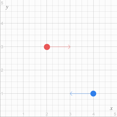
Then in vector form it can be represented as follows:

If we combine all this into one vector, we will get what we need
:
Derived function
determines the initial state and now all we need is to find a way to transition from the initial state to the state that occurs the instant after it, and from the received state a little further in time and so on. To do this, solve the equation
for . Find the derivative of:
Wow! The formula turned out high! But you can bring it into a more readable form if we break our vector
back to the component parts.
 and
and  bound by similar rules, as well as
  from
from  , so despite the bunch of expressions above, all we really need to find are the following 2 things:
The quality of the simulation depends on the definition of these two derivatives, it is in them all the strength. And so that the simulation does not resemble a program where everything happens in a chaotic way, you can turn to physics for inspiration.
Kinematics and Dynamics
Kinematics and dynamics are essential ingredients to create an interesting simulation. Let's start with the very basics in our example.
Responsible for the position in space
, and the first derivative of the point’s position in time is its velocity . In turn, the derivative of speed over time is acceleration, .
. It may seem that we have already found the function we need
because we already know the following:
And in fact, we brilliantly dealt with
 because this is part of our state vector
  , but we need to make out the second formula a little more, because with not so simple.
 Here Newton’s second law will help us:
 . If we assume that the mass of our objects is known, then rearranging the variables in the expression, we get:
So wait a minute
and  are not part , so it’s hard to call promotion (remember, we need a derivative function that depends only on and
  ) Nevertheless, we moved forward, because we found all the useful formulas that determine the behavior of objects in our physical world.
 Suppose that in our simple example, the only force that acts on objects is gravitational attraction. In this case, we can determine
using Newton’s law of gravity:
Where
 this is the gravitational constant
  , a
, a  and
and  these are the masses of our objects (which, we assume, are constants).
 To create the simulation itself, we also need a direction and somehow indicate
 through vector components . Assuming that
 is the force acting on the first object, then we can do it as follows:
![$ \ begin {aligned} \ vec F_1 & = G \ frac {m_1 m_2} {| \ vec x_2 - \ vec x_1 | ^ 2} \ left [\ frac {\ vec x_2 - \ vec x_1} {| \ vec x_2 - \ vec x_1 |} \ right] = G \ frac {m_1 m_2 (\ vec x_2 - \ vec x_1)} {| \ vec x_2 - \ vec x_1 | ^ 3} \\ \\ \ vec F_2 & = G \ frac {m_2 m_1} {| \ vec x_1 - \ vec x_2} {| \ vec x_1 - \ vec x_2} {| \ vec x_1 - \ vec x_2 |} \ right] = G \ frac {m_2 m_1 (\ vec x_1 - \ vec x_2)} {| \ vec x_1 - \ vec x_2 | ^ 3} \ end {aligned} $](https://habrastorage.org/getpro/habr/formulas/b59/139/df7/b59139df72b4abdec9d98404d75c288a.svg)
To summarize. The change of states in our system of two objects is fully expressed through variables
 . And the changes are:
Now we have everything that distinguishes our simulation from all other simulations:
and .
But how, having a strictly defined simulation, turn it into a beautiful animation?
If you had experience writing a simulation or a game, then maybe you can suggest something like this:
x += v * delta_t
v += F/m * delta_t
But let's stop a bit and see why this works.
Differential equations
Before we begin implementation, we need to decide what information we already have and what we need. We have a meaning
which satisfies there is also satisfying  . And we need a function that will give us the state of the system at any time. Mathematically, we need a function.
 Bearing this in mind and looking closely at
, you can see that this equation relates  with its derivative
  . This means that our equation is differential! Ordinary differential equation of the first order, to be precise. If we solve it, then we will find a function.
 The task of finding
according to and called the Cauchy problem .Numerical integration
For some examples of Cauchy problems, you can easily find the answer by the analytical method, but in complex simulations the analytical approach can be very difficult. Therefore, we will try to find a way to find an approximate solution to the problem.
For example, take the simple Cauchy problem.
Given:
 and
and  . Find an approximate solution for.
 Consider the problem from a geometric point of view and look at the value and tangent at a point
 . From what is given to us, we have and
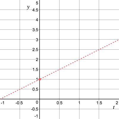
We don’t know what it looks like
but we know that near the point , the value is close to the tangent. Now try to calculate for small value
  using the tangent. Let's try for a start
 .
.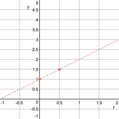
If you paint, then we approximate the value
 in the following way:
So, for
 .
Now we can continue to be calculated for other points. Although, of course, we did not find the exact valuebut if our approximate value is very close to exact, then the approximated tangent will also be very close to real!
.
Now we can continue to be calculated for other points. Although, of course, we did not find the exact valuebut if our approximate value is very close to exact, then the approximated tangent will also be very close to real!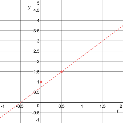
Next, let's move on
units to the right tangent.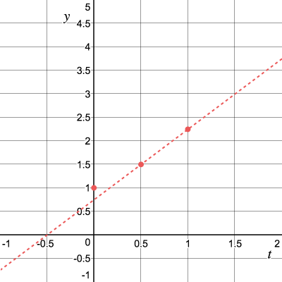
Repeat the process and get the tangent slope
 :
: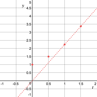
The procedure can be performed recursively and for this we derive the formula:

This numerical method for solving differential equations is called the Euler method. For the general case, a step
x += v * delta_t. In our particular case, a step-by-step solution looks like this:

Using this method, it is convenient to present the results in a table:

It turns out that our problem has a beautiful analytical solution
 :
:
What do you think will happen if the step is reduced in the Euler method?
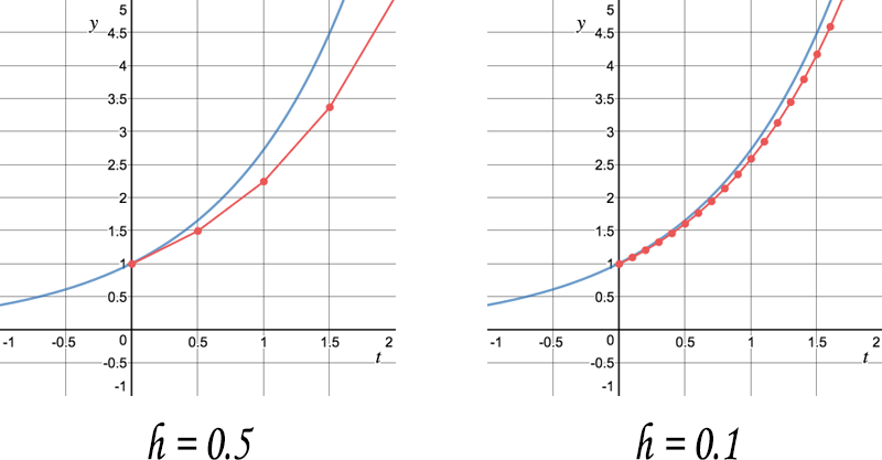
The difference between approximated and exact solutions decreases with decreasing
! In addition, in addition to reducing the step, other methods of numerical integration can be used, which can lead to a better result, such as the middle rectangle method , the Runge-Kutta method, and the Adams method .It is time to code!
With the same success as we deduced the mathematical representation of the description of the simulation, we can write the implementation of the simulation programmatically.
Because I am most familiar with JavaScript, and I like the clarity that annotations add to the code, all examples will be written in TypeScript .
And we will start with the version, which implied that
it is a one-dimensional array of numbers, just like in our mathematical model. function runSimulation(
// y(0) = y0
y0: number[],
// dy/dt(t) = f(t, y(t))
f: (t: number, y: number[]) => number[],
// показывает текущее состояние симуляции
render: (y: number[]) => void
) {
// Шаг вперёд на 1/60 секунды за тик
// Если анимация будет 60fps то это приведёт к симуляции в рельном времени
const h = 1 / 60.0;
function simulationStep(ti: number, yi: T) {
render(yi)
requestAnimationFrame(function() {
const fi = f(ti, yi)
// t_{i+1} = t_i + h
const tNext = ti + h
// y_{i+1} = y_i + h f(t_i, y_i)
const yNext = []
for (let j = 0; j < y.length; j++) {
yNext.push(yi[j] + h * fi[j]);
}
simulationStep(tNext, yNext)
}
}
simulationStep(0, y0)
}It is not always convenient to operate with one-dimensional arrays; you can abstract the functions of adding and multiplying the simulation process into an interface and get a brief generalized simulation implementation using TypeScript Generics .
interface Numeric {
    plus(other: T): T
    times(scalar: number): T
}
function runSimulation>(
  y0: T,
  f: (t: number, y: T) => T,
  render: (y: T) => void
) {
    const h = 1 / 60.0;
    function simulationStep(ti: number, yi: T) {
        render(yi)
        requestAnimationFrame(function() {
            // t_{i+1} = t_i + h
            const tNext = ti + h
            // y_{i+1} = y_i + h f(t_i, y_i)
            const yNext = yi.plus(f(ti, yi).times(h))
            simulationStep(yNext, tNext)
        })
    }
    simulationStep(y0, 0.0)
}
The positive side of this approach is the ability to concentrate on the basis of the simulation: what exactly distinguishes this simulation from any other. We use the simulation example with the two objects mentioned above:
Code simulation of two objects
// Состояние симуляции двух объектов в один тик времени
class TwoParticles implements Numeric {
    constructor(
        readonly x1: Vec2, readonly v1: Vec2,
        readonly x2: Vec2, readonly v2: Vec2
    ) { }
    plus(other: TwoParticles) {
        return new TwoParticles(
            this.x1.plus(other.x1), this.v1.plus(other.v1),
            this.x2.plus(other.x2), this.v2.plus(other.v2)
        );
    }
    times(scalar: number) {
        return new TwoParticles(
            this.x1.times(scalar), this.v1.times(scalar),
            this.x2.times(scalar), this.v2.times(scalar)
        )
    }
}
// dy/dt (t) = f(t, y(t))
function f(t: number, y: TwoParticles) {
    const { x1, v1, x2, v2 } = y;
    return new TwoParticles(
        // dx1/dt = v1
        v1,
        // dv1/dt = G*m2*(x2-x1)/|x2-x1|^3
        x2.minus(x1).times(G * m2 / Math.pow(x2.minus(x1).length(), 3)),
        // dx2/dt = v2
        v2,
        // dv2/dt = G*m1*(x1-x1)/|x1-x2|^3
        x1.minus(x2).times(G * m1 / Math.pow(x1.minus(x2).length(), 3))
    )
}
// y(0) = y0
const y0 = new TwoParticles(
    /* x1 */ new Vec2(2, 3),
    /* v1 */ new Vec2(1, 0),
    /* x2 */ new Vec2(4, 1),
    /* v2 */ new Vec2(-1, 0)
)
const canvas = document.createElement("canvas")
canvas.width = 400;
canvas.height = 400;
const ctx = canvas.getContext("2d")!;
document.body.appendChild(canvas);
// Текущее состояние симуляции
function render(y: TwoParticles) {
    const { x1, x2 } = y;
    ctx.fillStyle = "white";
    ctx.fillRect(0, 0, 400, 400);
    ctx.fillStyle = "black";
    ctx.beginPath();
    ctx.ellipse(x1.x*50 + 200, x1.y*50 + 200, 15, 15, 0, 0, 2 * Math.PI);
    ctx.fill();
    ctx.fillStyle = "red";
    ctx.beginPath();
    ctx.ellipse(x2.x*50 + 200, x2.y*50 + 200, 30, 30, 0, 0, 2 * Math.PI);
    ctx.fill();
}
// Запускаем!
runSimulation(y0, f, render)
If you play with numbers, you can get a simulation of the orbit of the moon!
Simulation of the orbit of the moon, 1 pix. = 2500 km. 1 sec Simulation is 1 day on Earth. The proportion of the moon to the earth is increased 10 times
Collisions and restrictions
The above mathematical model actually simulates the physical world, but in some cases, the method of numerical integration, unfortunately, breaks down.
Imagine a simulation of a ball bouncing on the surface.
The simulation state can be described as follows:

Where
 this is the height of the ball above the surface, and
  his speed. If you release the ball from a height of 0.8 meters, we get:
If you plot
 then we get something like the following:
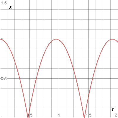
Derivative function during ball fall
easy to compute:
With the acceleration of gravity,
 .
. But what happens when the ball touches the surface? That the ball has reached the surface we can find out by
 . But with numerical integration, at one point in time, the ball can be above the surface, and already at the next below it:
 .
. This problem could be solved by determining the moment of collision
 . But even if this moment is found, how to determine the acceleration
 so that it changes in the opposite direction.
 You can, of course, determine the collision in a limited period of time and apply another force
 for this length of time
  , but it’s much easier to define a discrete constant limiting simulation.
 And in order to reduce the amount of penetration by the ball of the surface, it is possible to calculate several simulation steps in one tick at once. Together with this, the code of our simulation will change like this:
function runSimulation>(
  y0: T,
  f: (t: number, y: T) => T,
  applyConstraints: (y: T) => T,
  iterationsPerFrame: number,
  render: (y: T) => void
) {
    const frameTime = 1 / 60.0
    const h = frameTime / iterationsPerFrame
    function simulationStep(yi: T, ti: number) {
        render(yi)
        requestAnimationFrame(function () {
            for (let i = 0; i < iterationsPerFrame; i++) {
                yi = yi.plus(f(ti, yi).times(h))
                yi = applyConstraints(yi)
                ti = ti + h
            }
            simulationStep(yi, ti)
        })
    }
    simulationStep(y0, 0.0)
}
And now you can write the code of our bouncing ball:
Bouncing ball code
const g = -9.8; // m / s^2
const r = 0.2; // m
class Ball implements Numeric {
    constructor(readonly x: number, readonly v: number) { }
    plus(other: Ball) { return new Ball(this.x + other.x, this.v + other.v) }
    times(scalar: number) { return new Ball(this.x * scalar, this.v * scalar) }
}
function f(t: number, y: Ball) {
    const { x, v } = y
    return new Ball(v, g)
}
function applyConstraints(y: Ball): Ball {
    const { x, v } = y
    if (x <= 0 && v < 0) {
        return new Ball(x, -v)
    }
    return y
}
const y0 = new Ball(
    /* x */ 0.8,
    /* v */ 0
)
function render(y: Ball) {
    ctx.clearRect(0, 0, 400, 400)
    ctx.fillStyle = '#EB5757'
    ctx.beginPath()
    ctx.ellipse(200, 400 - ((y.x + r) * 300), r * 300, r * 300, 0, 0, 2 * Math.PI)
    ctx.fill()
}
runSimulation(y0, f, applyConstraints, 30, render)
Attention to the developers!
Although this model has its advantages, it does not always lead to productive simulations. For me, such a framework is useful for representing the behavior of a simulation, even if a lot of unnecessary things happen in it.
For example, the rain simulation at the beginning of this article [ approx. In the original article, a beautiful interactive rain simulation was inserted at the beginning, I recommend that you look first-hand] was not created using the template described in the article. It was an experiment using Entity – component – system . The simulation source can be found here: rain simulation on GitHub .
See you later!
I find the intersection of mathematics, physics, and programming something really impressive. Creating a working simulation, running it and rendering it is a special kind of something out of nothing .
All of the above was inspired by the materials of the SIGGRAPH lecture, just like in the fluid simulation . If you want to find more comprehensive information about the above, then take a look at the materials of the SIGGRAPH 2001 course "Introduction to Physical Modeling" . I give a link to the 1997 course, as Pixar seems to have removed version 2001.
I want to thank Maggie Cai for the wonderful illustration of the couple under the umbrella and for their patience with painstaking selection of colors, while I can not distinguish between blue and gray.
And if you are interested, then the illustrations were created in Figma .
Only registered users can participate in the survey. Please come in.
Whether to translate the article “fluid simulation” (the link is given in the conclusion of the article)
- 96.8% Yes 154
- 3.1% No 5