Learn OpenGL. Lesson 2.5 - Light Sources
- From the sandbox
- Tutorial

Sources of light
Until this article, we were content with lighting coming from one point in space. And the result was not bad, but in reality there are many sources of illumination with different "behavior". This lesson discusses several of these light sources. The ability to imitate the characteristics of different light sources is another tool to enrich the created scenes.
We start the lesson with a directional light source, then move on to a point source, which is a development of the mentioned simple lighting method. In the end, we will consider how the source is constructed that imitates the properties of a spotlight (spotlight).
Content
Part 1. Getting Started
Part 2. Basic lighting
Part 3. Download 3D models
Part 4. Advanced OpenGL Features
Part 5. Advanced Lighting
Part 6. PBR
- Opengl
- Window creation
- Hello window
- Hello triangle
- Shaders
- Textures
- Transformations
- Coordinate systems
- Camera
Part 2. Basic lighting
Part 3. Download 3D models
Part 4. Advanced OpenGL Features
- Depth test
- Stencil test
- Color mixing
- Clipping faces
- Frame buffer
- Cubic cards
- Advanced data handling
- Advanced GLSL
- Geometric shader
- Instancing
- Smoothing
Part 5. Advanced Lighting
- Advanced lighting. Blinn-Fong model.
- Gamma correction
- Shadow cards
- Omnidirectional shadow maps
- Normal mapping
- Parallax mapping
- HDR
- Bloom
- Deferred rendering
- SSAO
Part 6. PBR
Directional light source
If the light source is significantly removed from the object of observation, then the incoming rays of light turn out to be almost parallel to each other, giving the impression that the light is directed equally regardless of the location of the object and / or observer. The simulated infinitely distant light source is called directional, since all its rays are considered to go in the same direction and do not depend on the location of the source itself.
A good example of this type of source is our Sun. Although it is not infinitely distant from us, this distance is enough to consider it infinitely distant in lighting calculations. And assume that the rays of sunlight are parallel, as shown in the figure:

Since we consider the rays parallel, the relative position of the illuminated object and the source is not important - the direction of the rays will be the same throughout the scene. Accordingly, the calculation of lighting will be the same for all objects, since the vector of the direction of lighting is the same for any object in the scene.
To simulate a directional source, we can be given a lighting direction vector, and the position vector becomes unnecessary. Computing model in the shader remains practically constant: the calculation is replaced by a source direction vector lightDir using the source position vector on the direct use of the specified direction vector direction .
struct Light {
    // vec3 position; //Не требуется для направленного источника.
    vec3 direction;
    vec3 ambient;
    vec3 diffuse;
    vec3 specular;
};
...
void main()
{
  vec3 lightDir = normalize(-light.direction);
  ...
}
Note the inverse of the light.direction vector . Until now, the calculation model has accepted the direction vector of the light source as oriented from the fragment to the source , however, for directed sources, the direction vector is usually specified as oriented from the source . Therefore, an inversion is performed, and in a variable we save a vector directed to the light source. Also do not forget about normalization - it is better not to hope that the input data will be normalized.
So, in the end, lightDir is used in the calculations of the diffuse and mirror components in the same way as before.
In order to clearly demonstrate that a directional source equally affects the illumination of many objects, we will use the familiar scene code with a crowd of containers from the final of the Coordinate Systems lesson . For those who missed: first we set 10 different positions of the containers and assigned each of them a unique model matrix that stores the corresponding transformations from the local coordinate system to the world:
for(unsigned int i = 0; i < 10; i++)
{
    glm::mat4 model(1.);
    model = glm::translate(model, cubePositions[i]);
    float angle = 20.0f * i;
    model = glm::rotate(model, glm::radians(angle), glm::vec3(1.0f, 0.3f, 0.5f));
    lightingShader.setMat4("model", model);
    glDrawArrays(GL_TRIANGLES, 0, 36);
}
Also, do not forget to transfer the direction of our directional source to the shader (once again I remind you that we set the direction from the source; by the type of vector you can determine that it is directed down):
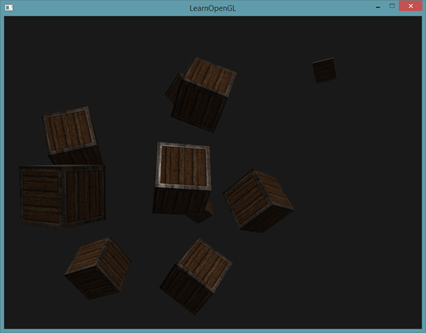
lightingShader.setVec3("light.direction", -0.2f, -1.0f, -0.3f);So far, we have transmitted positions and directions as three-component vectors ( vec3 ), however, some developers prefer the transfer in the form of vectors with four components ( vec4 ). When setting positions using vec4, it is extremely important to set the w component to 1 so that the transfer transforms and projection transforms are correctly applied. At the same time, when specifying directions in the form of vec4, we would not want the transfer to affect the direction (this is also the direction vector, after all), and therefore we must set w = 0 .If we now assemble our application, then moving around the stage, you will notice that all objects are illuminated by a source similar to the sun in its behavior. You see how the diffuse and mirror component of lighting on objects changes as if a source of light is located somewhere in a conditional sky? The results should be something like this:
Thus, the direction vector is represented as vec4 (0.2f, 1.0f, 0.3f, 0.0f). Such a record can also be used for an accessible check on the type of light source and the choice of a lighting calculation model: if the component w is 1, then this is clearly the position vector of the light source, if w is 0, then we have a direction vector:if(lightVector.w == 0.0) // обратите внимание на ошибки округления // выполнить расчет освещения для направленного источника else if(lightVector.w == 1.0) // выполнить расчет освещения с учетом положения источника // (как в предыдущем уроке)
Fun fact: this is how OpenGL defined a light source as directional or positioned and changed the calculation model during the fixed-functionality pipeline.
The source code for the example can be found here .
Point sources
Directional light sources do a good job of lighting the whole scene, but usually we need to place a few more point sources in the space of the scene. A point light source has a predetermined position in space and emits uniformly in all directions, and the light intensity decreases with distance. Conventional incandescent lamps or torches can be cited as an example of point sources.

In previous lessons, we used the simplest implementation of a point source with a given position, spreading light in all directions. However, the rays of this source did not fade away, which made the source look extremely powerful. In most scenes created, it would be desirable to have sources that affect the environment in close proximity to them, but not the whole scene at once.
If you add 10 containers to the scene of the previous example, you will notice that even the most remote of them are lit with the same intensity as those located directly in front of the source. And this is expected - we did not enter into account any expressions that control the intensity of lighting. But we want the remote containers to be only slightly highlighted compared to those closest to the source.
Attenuation
Attenuation of light intensity with distance is called attenuation. The simplest method of calculating attenuation is to use a linear law. In this case, the intensity will decrease linearly with distance, providing less illumination of distant objects. But visually such a model gives unrealistic results. In the general case, real light sources give strong illumination near, but the intensity decreases quite sharply in a small radius and then its remaining supply slowly decreases with distance. To simulate such behavior, you need a calculation more linear.
Fortunately, physicists are on the alert, and a generalized expression for calculating the attenuation coefficient from a distance has long been deduced. It remains only to calculate the value for each fragment and multiply by the result the intensity vector of a particular source:

 - the distance from the fragment to the source,
  - constant, linear and quadratic coefficients.
- As usual, the constant coefficient is 1.0, protecting against a decrease in the denominator to values less than unity, which would lead to an increase in the intensity of illumination at certain distances. For us, this effect is undesirable.
- A linear coefficient defines a term that linearly decreases the light intensity with increasing distance.
- The quadratic coefficient determines the term that defines the quadratic decrease in intensity. At small distances, the contribution of the quadratic term will be blocked by the contribution of the linear, but with increasing distance will become dominant in the expression.
The combination of linear and quadratic dependences allows you to create an effect when the intensity decreases linearly near the source, and after a certain distance of removal begins to decline much faster. As a result, the brightness of the source is large near, decreases rather quickly with increasing distance, and decreases more slowly at large distances. The following graph shows an example of the attenuation coefficient over 100 distance units:

As you can see, the intensity is greatest at short distances, but with growth it drops significantly and tends to zero in the vicinity of 100 units.
Odds selection
The question arises of choosing three coefficients
. Suitable values are sought based on the environment being developed in the scene, the required lighting distance, the type of source, and other factors. In most cases, this becomes a matter of experience and a certain amount of adjustment by trial and error. The table below contains a list of parameters that provide realistic, in a certain sense, the behavior of a light source covering a specified distance. The first column indicates the coverage distance at the set ratios. The table is taken from the project wiki page of the Ogre3D engine and is an excellent starting point for selecting the values you need.| Distance | Constant | Linear | Quadratic |
|---|---|---|---|
| 7 | 1.0 | 0.7 | 1.8 |
| thirteen | 1.0 | 0.35 | 0.44 |
| 20 | 1.0 | 0.22 | 0.20 |
| 32 | 1.0 | 0.14 | 0.07 |
| fifty | 1.0 | 0.09 | 0.032 |
| 65 | 1.0 | 0.07 | 0.017 |
| 100 | 1.0 | 0.045 | 0.0075 |
| 160 | 1.0 | 0.027 | 0.0028 |
| 200 | 1.0 | 0.022 | 0.0019 |
| 325 | 1.0 | 0.014 | 0.0007 |
| 600 | 1.0 | 0.007 | 0.0002 |
| 3250 | 1.0 | 0.0014 | 0.000007 |
As you can see, the constant coefficient is everywhere equal to unity. The linear coefficient is chosen small when illuminating large distances, and the quadratic coefficient is even smaller. Try to experiment with these values and personally see what effect their change has in the conditions of your implementation. For the scenes under consideration, the coating distance is from 32 to 100 units. quite enough.
Implementation
To implement the attenuation, we need three additional parameters in the fragment shader code: actually, constant, linear and quadratic coefficients. It is most logical to store them in the declared Light structure , which we used earlier. Please note that the calculation of the lightDir vector is carried out similarly to the previous lesson, and not the path described in the directional light source section.
struct Light {
    vec3 position;
    vec3 ambient;
    vec3 diffuse;
    vec3 specular;
    float constant;
    float linear;
    float quadratic;
};
Next, set the specific parameter values in the code. We need a lighting distance of about 50 units, for which the following values are indicated in the table:
lightingShader.setFloat("light.constant",  1.0f);
lightingShader.setFloat("light.linear",    0.09f);
lightingShader.setFloat("light.quadratic", 0.032f);
The calculation code in the fragment shader is obvious: we calculate the attenuation coefficient and then multiply the background, diffuse and mirror components of lighting by it.
For calculations, however, we need the value of the distance from the fragment to the light source. How do we get it? It's simple: just calculate the difference between the position vectors of the fragment and the source, and use the built-in GLSL length () function :
float distance    = length(light.position - FragPos);
float attenuation = 1.0 / (light.constant + light.linear * distance +
    		    light.quadratic * (distance * distance));
As a result, we multiply the resulting coefficient by all components of the lighting model.
It would be possible to leave the background component without attenuation, however, in scenes with several sources, the contribution of this component will begin to add up, which is usually undesirable. In this case, attenuation should be included for the background component.
ambient  *= attenuation;
diffuse  *= attenuation;
specular *= attenuation;
Running a test application, you can expect something like this:
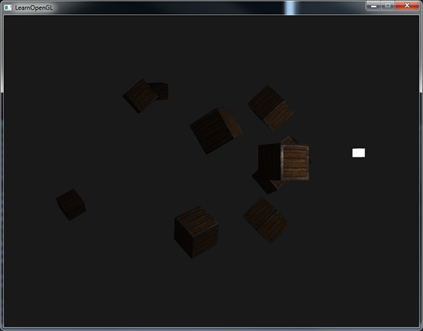
It can be seen that now only the containers in front are highlighted, and the nearest is the brightest. The containers in the back of the stage are not lit at all, because they are too far from the source.
The full example code can be found here . Summing up, we can say that a point source is a source with an adjustable position and taking into account the attenuation of the intensity in the lighting calculations. Another tool in our piggy bank!
Floodlight
The last source type considered will be a spotlight. Such a source has a predetermined position, but radiates not in all directions, but only in the selected one. At the same time, objects are illuminated only in a small neighborhood from a given direction, and objects lying outside this area remain without illumination. As an example, imagine a street lamp or a flashlight.
In our model, the spotlight will be represented by the position in world coordinates, the direction vector and the cutoff angle , which determines the radius of the spotlight backlight. To determine if a fragment is highlighted or not, we will calculate whether it is inside or outside the cone-shaped source clipping zone. This scheme will help you figure out how everything works:

Here, LightDir is the vector directed from the fragment to the source, SpotDir is the spotlight direction vector,
 ( phi ) - clipping angle defining the radius of the backlight (fragments lying outside this angle will not be highlighted),
 ( theta ) - the angle between the LightDir and SpotDir vectors (if less than , then the fragment falls into the backlight area).
 Thus, all that needs to be done is to calculate the scalar product of the LightDir and SpotDir vectors and compare the obtained value with the given clipping angle (with the cosine of the angle, because scalar multiplication returns the cosine of the angle between two normalized vectors). Now that you have a basic understanding of the searchlight, you can move on to implementation.
Implementation
We bring the model to life in the form of a flashlight, i.e. a source fixed at the point of position of the observer and directed straight ahead from his point of view. In fact, a flashlight is a source of the type of a searchlight, with the position and direction rigidly attached to the position and orientation of the player.
For transmission to the shader, we need position values (to calculate the vector to the light source), the direction vector of the spotlight, and the cutoff angle. All this can be placed in the Light structure :
struct Light {
    vec3  position;
    vec3  direction;
    float cutOff;
    ...
};
Next, we transfer the data to the shader in the program code:
lightingShader.setVec3("light.position",  camera.Position);
lightingShader.setVec3("light.direction", camera.Front);
lightingShader.setFloat("light.cutOff",   glm::cos(glm::radians(12.5f)));
As you can see, here we are transmitting not the cutoff angle, but its cosine, since in the shader we calculate the scalar product of vectors, which returns the cosine of the angle between them. In order to avoid calculating the cosine angle by calling the expensive acos () function, we will pass the finished cosine of the cut-off angle to the shader and we will directly compare these values, saving a little computing resources.
Actually, we will calculate and determine whether we are inside the coverage area of the spotlight or not:
float theta = dot(lightDir, normalize(-light.direction));
if(theta > light.cutOff)
{
  // расчет освещения
}
// иначе используем только фоновую компоненту, чтобы сцена не была
// полностью черной вне конуса прожектора
else  color = vec4(light.ambient * vec3(texture(material.diffuse, TexCoords)), 1.0);
First, we compute the scalar product of the LightDir vectors and the inverted direction vector (since we need a vector directed to the source, not from it). Do not forget to normalize all used vectors!
You may be surprised to use the comparison character “>” instead of “<” in a conditional statement. It seems that theta should be less than the cut-off value so that the fragment is in the cone of action of the spotlight? That's right, but we are not comparing angles here, but their cosines. The cosine of 0 ° is 1, and 90 ° is 0. Take a look at the graph:Launching a test application will show that now only those fragments that lie inside the cone of action of the spotlight are highlighted:
Obviously, with the cosine value tends to 1 with decreasing angle, which explains why theta should be greater than the cutoff value. In this example, the clipping value is equal to the cosine of the angle of 12.5 °, which is 0.9978. Accordingly, the fragment will be in the backlight cone if theta value is in the interval from 0.9978 to 1.0.


The full example code is here .
The results, however, are not impressive. The hard, sharp edges of the highlighted area look especially unrealistic. Fragments that have fallen from the cone of the spotlight are shaded instantly, without a drop in brightness. It is more realistic to smoothly reduce the backlight intensity in the clipping zone.
Smooth attenuation
To implement a searchlight with soft edges of the backlight zone, we need to set the inner and outer cones of this zone. The inner cone can be determined based on the data discussed in the previous section. From its borders to the borders of the outer cone, the intensity should smoothly decay.
The outer cone is determined using the cosine of the angle of the solution of this cone. As a result, for a fragment in the interval between the boundaries of two cones, the illumination intensity in the interval between 0.0 and 1.0 should be calculated. Fragments lying in the inner cone are always illuminated with an intensity of 1.0, and those that fall outside the outer cone are not illuminated at all.
The parameter determining the smooth decline in intensity can be calculated using the following formula:

 Is the difference in the cosines of the angles defining the internal () and external (
 ) cones,
  - coefficient of light intensity for a given fragment.
 It can be difficult to imagine how this expression behaves, so consider a couple of examples:
| θ | Θ ° | ϕ (internal) | ϕ ° | γ (external) | γ ° | ε | I |
|---|---|---|---|---|---|---|---|
| 0.87 | thirty | 0.91 | 25 | 0.82 | 35 | 0.91 - 0.82 = 0.09 | 0.87 - 0.82 / 0.09 = 0.56 |
| 0.9 | 26 | 0.91 | 25 | 0.82 | 35 | 0.91 - 0.82 = 0.09 | 0.9 - 0.82 / 0.09 = 0.89 |
| 0.97 | 14 | 0.91 | 25 | 0.82 | 35 | 0.91 - 0.82 = 0.09 | 0.97 - 0.82 / 0.09 = 1.67 |
| 0.83 | 34 | 0.91 | 25 | 0.82 | 35 | 0.91 - 0.82 = 0.09 | 0.83 - 0.82 / 0.09 = 0.11 |
| 0.64 | fifty | 0.91 | 25 | 0.82 | 35 | 0.91 - 0.82 = 0.09 | 0.64 - 0.82 / 0.09 = -2.0 |
| 0.966 | fifteen | 0.9978 | 12.5 | 0.953 | 17.5 | 0.966 - 0.953 = 0.0448 | 0.966 - 0.953 / 0.0448 = 0.29 |
As you can see, this is a simple interpolation operation between the cosine of the outer and inner cutoff angle, depending on the value
. If even now it is not clear what is happening, then do not worry - you can simply take the formula as a given and return to it after a year by an experienced and wise person. One problem is value
now it turns out that there is less than zero in the region outside the outer cone, more than unity in the region of the inner cone, and intermediate values between the boundaries. It is necessary to correctly limit the range of values in order to get rid of the need for conditional operators and simply multiply the components of the lighting model by the calculated intensity value:float theta = dot(lightDir, normalize(-light.direction));
float epsilon = light.cutOff - light.outerCutOff;
float intensity = clamp((theta - light.outerCutOff) / epsilon, 0.0, 1.0);
...
// we'll leave ambient unaffected so we always have a little light.
diffuse *= intensity;
specular *= intensity;
...Pay attention to the clamp () function , which limits the range of values of its first parameter to the values of the second and third parameters. In this case, the value of intensity will lie on the interval [0, 1].
Do not forget to add the outerCutOff parameter to the Light structure and configure the transfer of a specific value to the uniform shader variable. For this image, the internal angle is set to 12.5 °, and the external - 17.5 °:
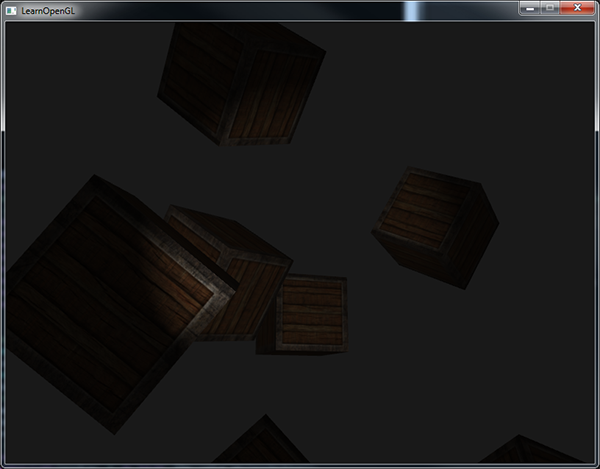
Much better! Now you can play with the settings of the clipping zones and get a spotlight that is ideally suited to your task. The source code of the application can be found here .
This type of flashlight source is ideal for horror games, and in combination with directional and point sources, the scenes you create will dramatically change.
In the next lesson, we will try to use all the types of sources and graphic techniques considered at the moment.
Tasks
Try experimenting with all the described types of sources and their fragment shaders. Invert some vectors and / or change the signs of comparisons. Understand for yourself the results of such actions.
Original article .