From two tuning forks from the Lissajous experiments to one elliptical level gauge tube with a step of a century and everything in Python

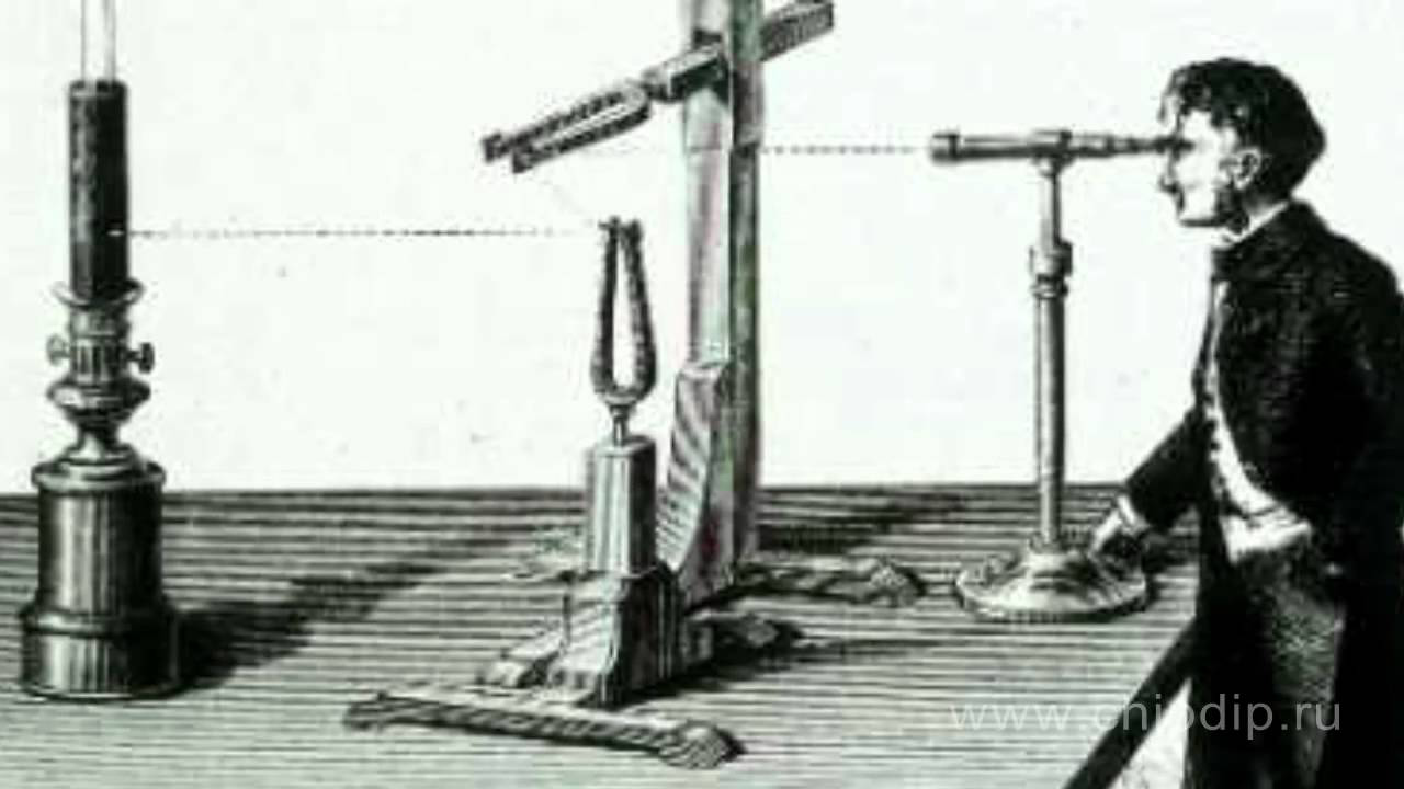
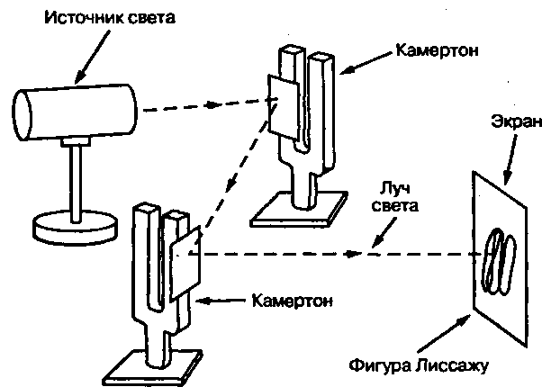
Pictures from the network, quality desires better, but they accurately reflect the essence of the experience in visualizing figures. Seeing the root is the foundation of the wisdom of generations.

A bit of history

Back in school, at physics lessons, I peered at an oscilloscope, on the screen of which, changing each other, various figures appeared: first simple ones - a line, a parabola, a circle, an ellipse, then the figures became more saturated with continuous wave-like lines reminding me of lace. The author of this lace diva was Jules Antoine Lissajous, a French physicist, a corresponding member of the Paris Academy of Sciences (1879) [1]. The figures themselves are closed trajectories drawn by a point that simultaneously performs two harmonic oscillations in two mutually perpendicular directions [2]. I think that in those years far from modern, the main merit of Jules, in addition to the knowledge of mathematics and physics, certainly accumulated by experience, was a simple mechanical visualization of these figures by improvised means. I wanted to design like Jules as simple and visual as possible, realize his ideas in relation to the modern task of linear measurements. But to do this by mathematical modeling with graphical visualization of its results in Python. But first, consider the classic version [3] of the construction of figures.

What should be the figures of Lissajous

To do this, we use the system of equations describing the figures:



x (t), y (t) in the general case, time-dependent harmonic oscillations along mutually perpendicular planes, frequencies b, a and the initial phase d. To analyze the figures in the calculations, the modulus of the frequency difference | b - a | = 1. We will consider the ratio of circular frequencies b / a and the initial phase d. We have for the line A = B d = 0, circles , and parabolas . We enter the main frequency relations satisfying the condition into the nested list m = [[0], [2,2], [2,1], [1,2], [3,2], [3,4], [5 , 4], [5,6], [9,8]].


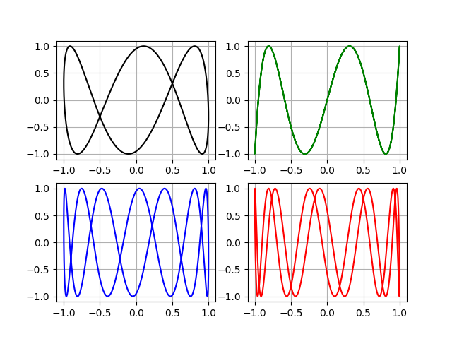
I don’t give the result, individual figures are not impressive. I want a collage of "lace".



And here they are "lace".

What can not be attributed to the Lissajous figures by definition of their isolation

Why do we need | b - a | = 1, “for the flags!” Let’s try, for example, m = [[1,3], [1,5], [1,7], [1,9]]



In the second graph, for m = 0,2, an open trajectory is obtained , which by definition is not a figure of Lbssazhu.

In search of mechanical analogues

Let's look for analogies of figures in measuring technique and here is a vibrational level gauge with a resonator in the form of an elliptical tube [4].

An elastically fixed tube of elliptical cross-section using self-excited systems 5,6,7 makes self-oscillations in one plane, and with the help of systems 8, 9, 10 in another plane perpendicular to the first. The tube oscillates in two mutually perpendicular planes with different frequencies close to their own. The mass of the tube depends on the level of the fluid filling it. With a change in mass, the tube oscillation frequencies also change, which are the output signals of the level gauge. The frequencies carry additional information about the multiplicative and additive additional errors compensated for when the frequencies are processed by the microprocessor 11.

Conditions for adequate modeling

To more or less correctly link the Lissajous figures to the work of the mentioned level gauge, the following circumstances should be taken into account. Firstly, an elliptical tube fixed at one end is an oscillatory system with distributed parameters, which greatly complicates the analysis of its oscillations. Secondly, the ratio of the tube oscillation frequencies cannot vary arbitrarily; it depends on the ellipse of the cross section and the permissible gaps in the oscillation excitation system. For the frequency ratio, you can get a simple ratio.



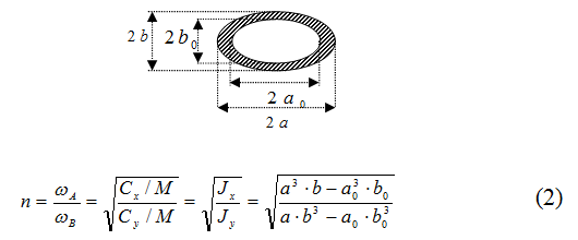
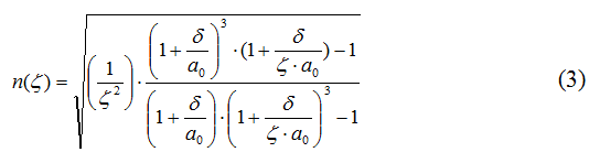
What the variables belong to, a, b, a0, b0 is clear from the figure, and in addition, the formula for the cyclic frequency of the oscillator is known from the school physics course. For “implementation in Python, in the last relation, we introduce the wall thickness and the ellipse index of the inner section of the tube, then instead of four variables we get three.





As a result of the program, we get a schedule.



The graph is built for a small internal axis of 9 mm. For a constructively permissible ratio of the small to the major semi-axis of the section in the range from 0.8 to 0.95. This is the main factor influencing the frequency ratio, which varies from 1.18 to 1.04. Wall thickness affects slightly. Now we have a range of relationships and can be used for further modeling.

Waveforms of the vertical axis of the tube

As for the distributed mechanical parameters of the cantilever tube, they can be reduced to the concentrated mass of stiffness and damping using the equality of natural frequencies and impedance. In addition, to determine the forms of bending vibrations of the cantilever tube, one can obtain an expression for distributed parameters. The equation for the forms - beam functions has the form:


where are the roots of the equation:


It should be noted that, despite a large number of publications on the forms and frequencies of oscillations of the cantilever rod, beam or tube, equations (4) are not given anywhere, only figures without coordinates. Therefore, I deduced equation (4) through the conditions at the ends and the beam functions, checked the roots (5) and the location of the nodes. However, this is a trivial equation that is simply forgotten.


As a result of the program, we get a graph built taking into account the vertical position of the tube.



On the graph, the coordinate of the axial line is reduced to the length of the tube, and the amplitude is normalized. The position of the vibration nodes of the tube relative to its mounting location exactly corresponds to the theory of oscillations.

What paths does the tube end

The last obstacle is the difficulty of obtaining a meaningful numerical solution of the differential equations of oscillations, provided that several parameters are varied simultaneously. Here, two of my articles on the vibrational link in Python [5,6] came to the rescue, in which a technique for obtaining exact symbolic solutions of differential equations is given.

We write two conditionally independent equations for tube oscillations in the OX and OY plane with different frequencies a and b, the relation between which is selected from a previously established range. The remaining parameters are selected in the correct relationship, but arbitrarily to better demonstrate the result.



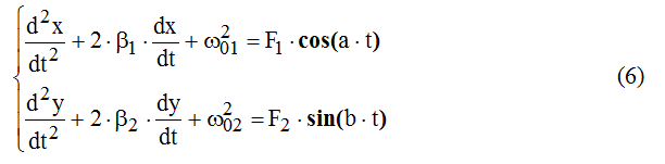
The following notation is introduced here (to simplify without indexes).

─ reduced amplitude of the force, ─ attenuation coefficient,─ the natural frequency of the system’s oscillations, m ─ the concentrated mass is the same for both equations, ─ the concentrated damping coefficients are different due to different amplitudes, and therefore different gaps in the excitation systems, ─ different stiffness due to the ellipticity of the tube section.


The program allows you to change all the parameters of the model, for example, for:
N = 1000, B = 0.2, f = 1, n1 = 0, n2 = 20, w1 = 5.0, w2 = 10.0, v1 = 0, v2 = 0


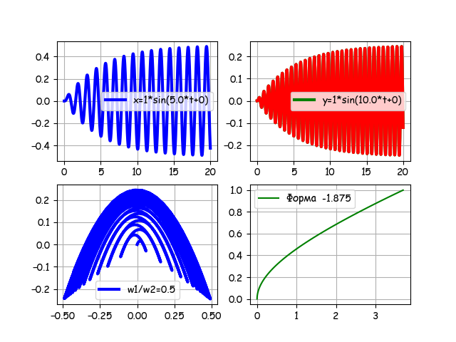
For a frequency ratio of 0.5 transient multiplies shapes. Put the “gate” of time n15 = 0, n2 = 20, we get.


We remove the “gate” and enter the initial phase v2 = -pi / 2, we get:


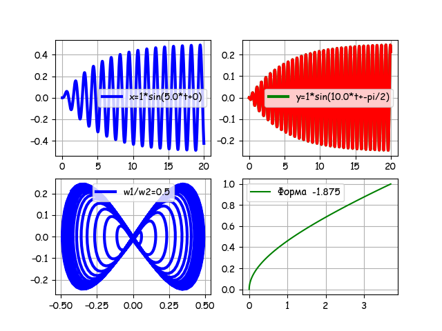
In view of the above, I do not require a comment on graphics.

For intrigue

If this article finds its readers or readers find it without fear of the shadows of the past, then I will publish three-dimensional animated graphics of complex spatial vibrations of the tube when the level of the filling fluid in it changes.

Instead of conclusions

The invention of Jules Antoine Lissajous continues his journey in time, but already in Python. I hope that the presented interpretation, of course far from perfect, will allow us to continue acquaintance with the works of the ingenious mathematician Lissajous.

References

1. Biographies of scientists physicists.
2. What are Lissajous figures?
3. Lissajous figures.
4. Vibrating level gauge.A.S.№777455
5. A model of the vibrational link using symbolic and numerical solutions of the differential equation in SymPy and NumPy.
6. The resonant link model in resonance mode in Python.