Recursive coordinate bisection method for decomposition of computational grids

Introduction

Calculation grids are widely used in solving numerical problems using finite difference methods. The quality of constructing such a grid to a large extent determines the success in the solution, so sometimes grids reach huge sizes. In this case, multiprocessor systems come to the rescue, because they allow you to solve 2 problems at once:

1. To increase the speed of the program.
2. Work with grids of a size that does not fit in the RAM of one processor.

With this approach, the grid covering the computational domain is divided into many domains, each of which is processed by a separate processor. The main problem here is the “honesty” of the partition: you need to choose a decomposition in which the computational load is distributed evenly between the processors, and the overhead caused by duplication of calculations and the need to transfer data between the processors is small.

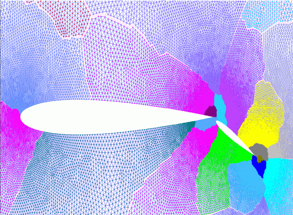
A typical example of a two-dimensional computational grid is shown in the first picture. It describes the space around the wing and flap of the aircraft, the grid nodes are condensed to small details. Despite the visual difference in the sizes of the multi-colored zones, each of them contains approximately the same number of nodes, i.e. we can talk about a good decomposition. This is the problem we will solve.

Note: since parallel sorting is actively used in the algorithm, it is highly recommended to know what the “ Exchange sorting network with the Butcher merge ” is to understand the article .

Formulation of the problem

For simplicity, we assume that our processors are single-core. Once again, to avoid confusion:
1 processor = 1 core . A computing system with distributed memory, so we will use MPI technology. In practice, in such systems, processors are multi-core, which means that threads should also be used for the most efficient use of computing resources.

We restrict the grids to only regular two-dimensional ones, i.e. such in which the node with indices (i, j) is connected to neighboring nodes existing in i, j: (i-1, j), (i + 1, j), (i, j-1), (i, j +1) . As you can see, the grid is not regular in the top picture, examples of regular grids are shown below:


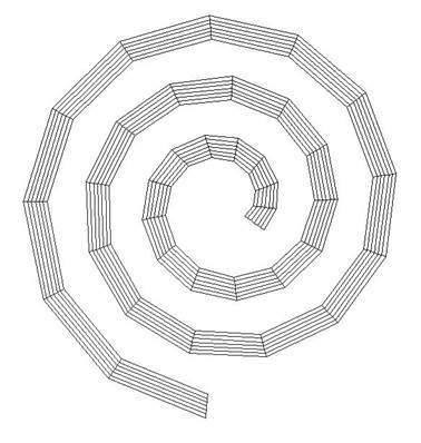
Thanks to this, the grid topology can be stored very compactly, which can significantly reduce both memory consumption and program runtime (after all, much less data needs to be sent over the network between processors).

The program receives 3 arguments to the input:

• n1, n2 - dimensions of a two-dimensional grid.
• k is the number of domains (parts) into which you want to split the grid.

The coordinates are initialized inside the program and, generally speaking, it doesn’t matter how it happens (you can see how this is done in the source code, a link to which is at the end of the article, but I will not dwell on this in detail).

We will store one grid node in the following structure:

struct Point{
    float coord[2]; // 0 - x, 1 - y
    int index;
};

In addition to the coordinates of the point, there is still an index of the node, which has 2 purposes. Firstly, it alone is enough to restore the grid topology. Secondly, it can be used to distinguish fictitious elements from normal ones (for example, for fictitious elements, set the value of this field to -1). About what these fictitious elements are and why they are needed, will be described in detail below.

The grid itself is stored in the Point P [n1 * n2] array , where the node with indices (i, j) is located in P [i * n2 + j] . As a result of the program, the number of vertices in the domains should be equal to one vertex with the value (n1 * n2 / k) .

Decision algorithm

The recursive coordinate bisection procedure consists of 3 steps:

1. Sort an array of nodes along one of the coordinate axes (in the two-dimensional case, along x or y).
2. Splitting a sorted array into 2 parts.
3. Recursive start of the procedure for the received subarrays.

The recursion basis here is the case k = 1 (1 domain remains). Something like this happens:

Or maybe so:


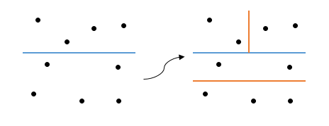
Where did the ambiguity come from? It is easy to see that I did not specify the criterion for choosing the axis, it was from here that different options appeared (in the first step, in the first case, the sorting takes place along the x axis, and in the second, along the y axis). So how to choose an axis?

1. Randomly.
   
   Cheap and cheerful, but takes only 1 line of code and requires a minimum of time. In the demo program, for simplicity, a similar method is used (in fact, there simply at every step the axis changes to the opposite, but from the conceptual point of view it is the same thing). If you want to write well - do not do so.
   
   
2. For geometric reasons.
   
   The length of the incision is minimized (in the general case, the incision is a hyperplane, so in the multidimensional case it’s more correct to talk about area). To do this, select the points with the minimum and maximum values ​​of the coordinates, and then measure the length based on some metric. Then it is enough to compare the obtained lengths and select the appropriate axis. Of course, it’s easy to pick up a counterexample here: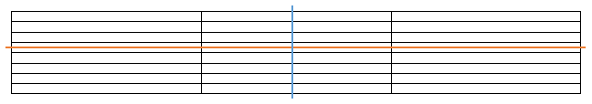
   
   
   
   The vertical section is shorter, but crosses 9 edges, while the longer horizontal section crosses only 4 edges. Moreover, such grids are not a degenerate case, but are used in problems. However, this option represents a balance between the speed and quality of the partition: it does not require as many calculations as in the third option, but the quality of the partition is usually better than in the first case.
   
   
3. Minimize the number of cut ribs.
   
   A split edge is an edge connecting vertices from different domains. Thus, if this number is minimized, then the domains are obtained as “autonomous” as possible, so we can talk about the high quality of the partition. So, in the picture above, this algorithm will select the horizontal axis. You have to pay for this with speed, because you need to sort the array along each axis, and then calculate the number of cut edges.

It’s worth mentioning how to split an array. Let m = n1 * n2 (the total number of nodes and the length of the array P ), and k the number of domains (as before). Then we try to divide the number of domains in half, and then divide the array in the same ratio. In the form of formulas:

int k1 = (k + 1) / 2;
int k2 = k - k1;
int m1 = m * (k1 / (double)k);
int m2 = m - m1;

For example: split 9 elements into 3 domains ( m = 9, k = 3 ). Then at first the array will be divided in a ratio of 6 to 3, and then the array of 6 elements will be split in half. As a result, we get 3 domains with 3 elements in each. What you need.

Note: some may ask why in the expression for m1 you need real arithmetic, because without using it you get the same result? The thing is overflow, for example, when breaking a grid of 10000x10000 into 100 domains m * k1 = 10 ¹⁰ , which is outside the range of int. Be careful!

Sequential algorithm

Having understood the theory, we can proceed to implementation. For sorting, we will use the qsort () function from the standard C language library. Our function will take 6 arguments:

void local_decompose(Point *a, int *domains, int domain_start, int k, int array_start, int n);

Here:

• a is the original mesh.
• domains - an output array in which domain numbers for grid nodes are stored (has the same length as array a ).
• domain_start - The starting index of the available domain numbers.
• k is the number of available items.
• array_start is the starting element in the array.
• n is the number of elements in the array.

First, we write the recursion basis:

void local_decompose(Point *a, int *domains, int domain_start, int k, int array_start, int n)
{
    if(k == 1){
        for(int i = 0; i < n; i++)
            domains[array_start + i] = domain_start;
        return;
    }

If we have only 1 domain left, then we put all available grid nodes into it. Then we select the axis and sort the grid along it:

    axis = !axis;
    qsort(a + array_start, n, sizeof(Point), compare_points);

The axis can be selected in one of the above ways. In this example, as mentioned earlier, it simply reverses. Here axis is a global variable that is used in the compare_points () element comparison function :

int compare_points(const void *a, const void *b)
{
    if(((Point*)a)->coord[axis] < ((Point*)b)->coord[axis]){
        return -1;
    }else if(((Point*)a)->coord[axis] > ((Point*)b)->coord[axis]){
        return 1;
    }else{
        return 0
    }
}

Now we just have to break down the domains and grid nodes available to us according to the corresponding formulas:

    int k1 = (k + 1) / 2;
    int k2 = k - k1;
    int n1 = n * (k1 / (double)k);
    int n2 = n - n1;

And write a recursive call:

    local_decompose(a, domains, domain_start, k1, array_start, n1);
    local_decompose(a, domains, domain_start + k1, k2, array_start + n1, n2);
}

That's all. The complete source code for the local_decompose () function is available on the github.

Parallel algorithm

Despite the fact that the algorithm has remained the same, its parallel implementation is much more complicated. I attribute this to two main reasons:

1) The system uses distributed memory, so each processor stores only its own part of the data without seeing the entire grid. Because of this, when dividing an array, you have to redistribute the elements.

2) As a sorting algorithm, Betcher’s parallel sorting is used, which requires that each processor has the same number of elements.

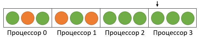
First, let's deal with the second problem. The solution is trivial - you need to introduce fictitious elements, which were mentioned in passing earlier. This is where the index field in the Point structure comes in handy.. We make it equal to -1 - and before us is a dummy element! Everything seems to be fine, but with this solution, we significantly exacerbated the first problem. In the general case, at the stage of dividing an array into 2 parts, it becomes impossible to determine not only the dividing element itself, but even the processor on which it is located. Let me explain this with an example: suppose we have 9 elements (3x3 grid) that need to be divided into 3 domains on 4 processors, i.e. n = 9, k = 3, p = 4. Then, after sorting, the dummy elements can appear anywhere (the grid nodes are green in the picture and the dummy elements are red):



In this case, the first element of the second array will be in the middle on the 2 processor. But if the dummy elements are arranged differently, then everything will change:



Here, the already breaking element was on the last processor. To avoid this ambiguity, we use a small hack: we will make the coordinates of dummy elements as possible (since they are stored in variables of type float in the program , the value will be FLT_MAX ). As a result, dummy elements will always be at the end:



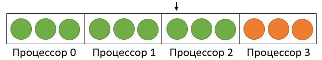
The picture clearly shows that with this approach, dummy elements will prevail on the latest processors. These processors will do useless work, sorting dummy elements at every step of the recursion. However, now the definition of the breaking element becomes a trivial task, it will be on the processor with the number:

int pc = n1 / elem_per_proc;

And have the following index in the local array:

int middle = n1 % elem_per_proc;

When the breaking element is determined, the processor containing it begins the process of redistributing the elements: it evenly distributes all elements to the breaking one to the processors “before” it (that is, with numbers smaller than it), adding dummy ones if necessary. He replaces the sent elements with dummy ones. In the pictures for n = 15, k = 5, p = 4:




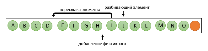
Now processors with numbers less than pc will continue to work with the first part of the original array, and the rest, in parallel, with the second part. At the same time, within the same group, the number of elements on all processors is the same (although the second group may have a different one), which makes it possible to further use Betcher sorting. Do not forget that the case pc = 0 is possible .- then it is enough to send the elements to the “other side”, ie to processors with large numbers.

The recursion basis in a parallel algorithm should be considered, first of all, the situation when we run out of processors: the case with k = 1 remains, but rather is degenerate, because in practice the number of domains is usually more than the number of processors.

Based on the foregoing, the general scheme of the function will look like this:

Conclusion

The considered implementation of the algorithm has a number of disadvantages, but at the same time it has an undeniable advantage - it works! The source code of the program can be found on the github . There is also an auxiliary utility for viewing the results. In preparing this article, the materials of the book by M. V. Yakobovsky "Introduction to parallel methods for solving problems" were used.