MEMS accelerometers and gyroscopes - we understand the specification
“Houston, we have a problem,” - tiredly sounded in the brain trying to wade through the Datasheet IMU MPU-9250 from InvenSense at night. When all words are separately understood, but their interrelation is confused to impossibility. It all started with the LSB parameter, about which I only vaguely remembered that the translation is Least Significant Bit. Then went “Resolution”, “Sensitivity”, and even further I realized that the resulting text can already be titled “Datasheet for dummies”.
It is a little about the main blocks of the inertial module.
The MPU-9250 consists of three independent uniaxial vibration angular velocity sensors (MEMS gyroscopes), which respond to rotation around the X, Y, and Z axes. Two suspended masses oscillate in opposite axes. With the advent of angular velocity, the Coriolis effect causes a change in the direction of the vibration (![$ \ vec {F} _K = -2m [\ vec {\ omega} \ times \ vec {v} _r] $](https://habrastorage.org/getpro/habr/formulas/caf/c87/5e3/cafc875e350a1c53728706f426e9614a.svg) which is fixed by a capacitive sensor. The measured differential capacitive component is proportional to the displacement angle [Electronics Time]. The resulting signal is amplified, demodulated and filtered, resulting in a voltage proportional to the angular velocity of rotation. This signal is digitized using the built-in 16-bit ADC board. The sample rate can programmatically vary from 3.9 to 8000 samples per second (samples per second, SPS), and user-defined low-pass filters (LPF) provide a wide range of possible cut-off frequencies. A low-pass filter is needed, including to remove vibrations from the motors (usually above 20-25 Hz).
which is fixed by a capacitive sensor. The measured differential capacitive component is proportional to the displacement angle [Electronics Time]. The resulting signal is amplified, demodulated and filtered, resulting in a voltage proportional to the angular velocity of rotation. This signal is digitized using the built-in 16-bit ADC board. The sample rate can programmatically vary from 3.9 to 8000 samples per second (samples per second, SPS), and user-defined low-pass filters (LPF) provide a wide range of possible cut-off frequencies. A low-pass filter is needed, including to remove vibrations from the motors (usually above 20-25 Hz).
For each axis, it uses a separate test mass, which is displaced when acceleration occurs along this axis (fixed by capacitive sensors). The MPU-9250 architecture reduces susceptibility to temperature drift and variations in electrical parameters. When the device is located on a flat surface, it will measure 0g along the X- and Y-axes and + 1g along the Z-axis. The scale factor (scale factor) is calibrated at the factory and does not depend on the supply voltage. Each sensor is equipped with an individual sigma-delta ADC (consists of a modulator and a digital low-pass filter, for more details about the device in [Easyelectronics]), the output digital signal of which has an adjustable measurement range.
Based on high-precision Hall effect technology. It includes magnetic sensors that determine the earth's magnetic field strength along axes, a control circuit, a signal amplification circuit, and a computational circuit for processing signals from each sensor. Each ADC has a resolution of 16 bits, the measurement range . To measure weak magnetic fields, either a unit in the SI microtesla system (μT) or gauss (Gs, GHS system) is used:
 , [Radiolotsman]).
Suppose our accelerometer is now working in the measurement range , that is, the full range of possible values will be
  . The corresponding voltage values are digitized by a 16-bit ADC, which can split the entire interval as much as possible into
 steps. The minimum increment that can be detected is just one step.
 . Here we must remember that the account is conducted from scratch, so that in fact the maximum measured value will be
 . That is, the larger the bits in the digital word ADC or DAC, the smaller the discrepancy will be. In this case, the sensitivity (sometimes called the scale factor, the sensitivity scale factor) of the sensor on a specific range will be determined as the ratio of the electrical output signal and the mechanical effect. Traditionally indicated for a signal frequency of 100 Hz and temperature
 For the MPU-9250, the sensitivity is
  steps for every g or
  (
( ,
,  ), for another IMU, BMI088 from Bosch Sensortec, the sensitivity of the gyroscope is calculated in the same way, and for the accelerometer it is used
  steps on each g.

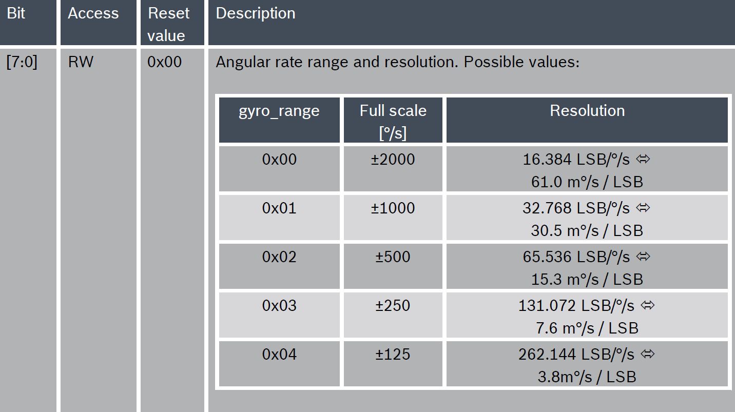
The FS options are taken out of the specification for gyroscopes and, in order not to get up twice, accelerometers.

I took FS for accelerometers also from the BMI088 documentation (see below).
Everything seems to fall into place, you can go further. In some cases (below, for example, a clipping from the documentation for BMI088), a parameter such as Resolution (Resolution) is separately indicated.
In fact, it seems, it turns out that it should be LSB. But why then do we see one value instead of several ones tied to specific ranges? I had to expand the list of investigated sources in search of answers.

The minimum value that the sensor reliably sees is extremely important when trying to strike a balance between price and performance. This is not an accuracy - a high-resolution sensor may not be particularly accurate, as well as a low-resolution sensor in certain areas may have sufficient accuracy. Unfortunately, LSB only defines a theoretical minimum distinguishable value, provided that we can use all 16 bits of the ADC. This resolution is in the digital world. In analog, some of the steps will be noisy and the number of effective bits will be less.
Noise sources can generally be broken down into electronic noise schemes that convert motion into a voltage signal (Johnson thermal noise, shot noise, pink 1 / f flicker noise, etc.), and thermal mechanical (Brownian, due to the presence of small moving parts) from the sensor itself. The characteristics of the latter will depend on the resonant frequency of the mechanical part of the system. (natural frequency of oscillation of the sensor
  ).
).
Noise levels can be determined in several ways. You can consider them in the time or frequency domain (after the Fourier transform). In the first case, the residual noise is taken as the rms value of the signals from the fixed sensor (in fact, this is the standard deviation for the sample at ) for a certain period of time:
Accelerations or angular rotational speeds below the level of broadband noise will be indistinguishable - that’s the actual resolution. The rms value of the ac voltage or current (often referred to as effective or effective) is equal to the magnitude of the constant signal, which will produce the same work in an active (resistive) load during a period. This approach is most effective in estimating broadband noise where white noise dominates.
For white noise, the ratio of the amplitude (instantaneous peak value) to the root mean square with a probability of 99.9% is Such an attitude is called the cross-factor (crest factor, cross ratio). You can choose the probability of 95.5% - the cross factor will be equal to 4.

In fact, noise signals behave not so well and can produce peaks that increase the cross factor up to 10 times. Some specifications may contain values. or the multiplier itself.
In the narrow low-frequency band of 0.1–10 Hz, the flicker noise “1 / f” plays the main role, for estimation of which the value of the peak-to-peak noise signal is used.
Sometimes it is more convenient to consider a signal in the frequency domain, where its description is called a spectrum (dependence of amplitude and phase on frequency). One of the possible noise characteristics in the specifications is called power spectral density of noise (PSD), noise spectral density, noise noise density, or simply noise density ). Describes the noise power distribution over a range of frequencies. Regardless of the representation of the electrical signal through the current or voltage, the instantaneous power dissipated in the load can be normalized (R = 1 Ohm) and expressed as Average power dissipated by a signal over a period of time
 can be written as
  , In general, these coefficients can be represented as follows:
  and
and  on frequency. Power spectral density
 periodic signal gives the distribution of signal power over the frequency range:
 ![$ [W / Hz] = [x ^ 2 / Hz]. $](https://habrastorage.org/getpro/habr/formulas/42c/1fb/e83/42c1fbe8340991ef020046242aabe392.svg) The average normalized power of the actual signal will be
The average normalized power of the actual signal will be  tends to infinity, the sequence of pulses turns into a separate pulse , the number of spectral lines tends to infinity, the spectrum graph turns into a smooth frequency spectrum
  For this limiting case, you can define a pair of Fourier integral transforms
  - Fourier-image.
The power spectral density of a random signal is determined through the limit
Since we assume that the average for the white noise of the sensors in a stationary state is zero ( ), then the square of the rms value is equal to the variance and represents the total power in the normalized load:
We look in the specification - there, in fact, under the name of the spectral density is indicated the square root of it with the corresponding dimension![$ [^ {\ circ} / s / \ sqrt {Hz}] $](https://habrastorage.org/getpro/habr/formulas/82b/0d2/43d/82b0d243d0b7d2ad1bee462c9825e4f5.svg) or
or ![$ [\ mu g / \ sqrt {Hz}]. $](https://habrastorage.org/getpro/habr/formulas/cf1/558/a68/cf1558a68250ba3a61f072d8964c2130.svg) That is, the RMS value of the noise without specifying the frequency band on which it was considered (Bandwidth) is meaningless.
That is, the RMS value of the noise without specifying the frequency band on which it was considered (Bandwidth) is meaningless.
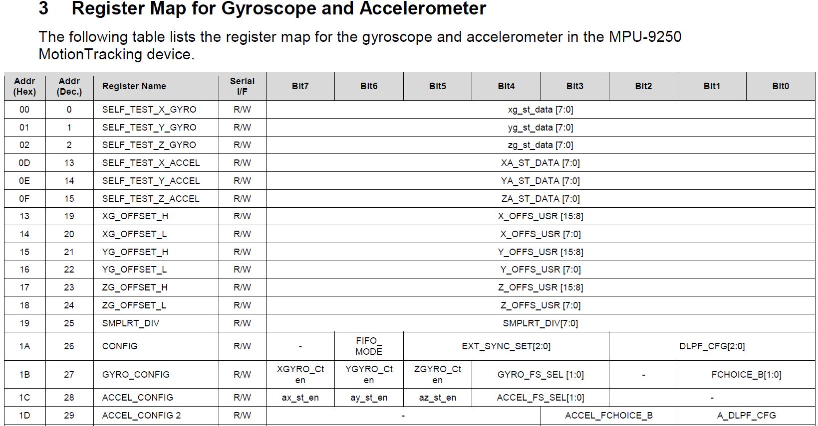
At the output of the MEMS sensor, we receive signals of different frequencies. It is assumed that we have in advance some idea of the processes we are measuring. For example, when determining the acceleration vector of a drone, the noise is the vibration of the apparatus. Separate them from the desired signal by using a low-pass filter, which cuts off all frequencies above that (for example, 200 Hz). The MPU-9250 provides the ability to adjust the cut-off frequency of the low-pass filter using the parameter with the magic name DLPFCFG. It stands for Digital Low Pass Filter Configuration. Further, in the specification, here and there, no less mysterious type expressions (DLPFCFG = 2, 92Hz) surfaced, but after decoding, I had to go into another document, “Register Map and Descriptions”. It shows which sets of bits in which registers need to be written to achieve the desired effects:
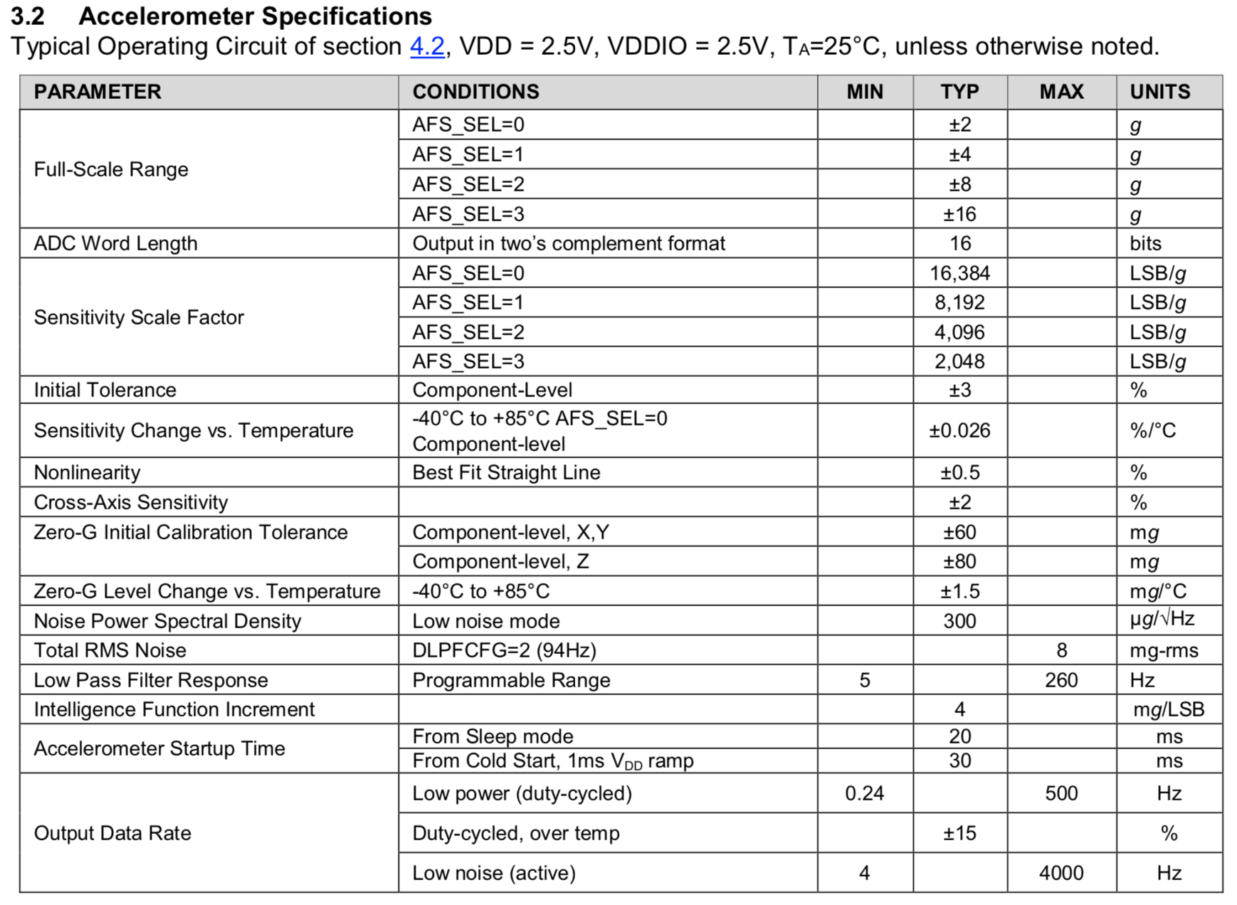
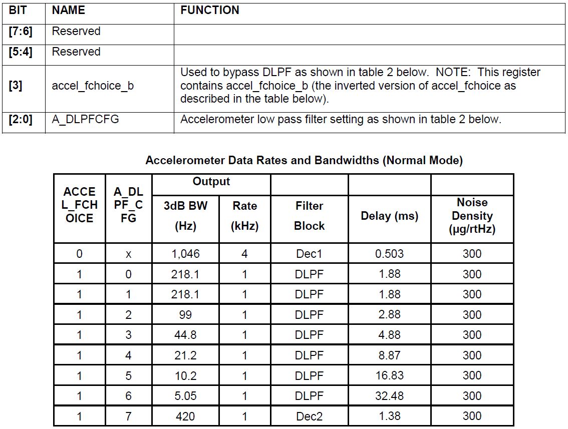
By omitting the technical details of the configuration, we can say the following. This sensor provides custom filtering of readings not only for accelerometers, gyros, but also for temperature sensors. For each, there are a total of 7 to 10 modes characterized by such concepts as Bandwidth in Hz, delay in ms, sampling frequency (Fs) in kHz.

The column “Noise density” was added to the accelerometer filter mode table in , and the “Bandwidth” column is supplemented with the value of “3dB”.
It did not get any easier, so let's go straight through the list.
Sample rate + decimation -ADC = data update rate (digital output data rate, ODR)
With the sampling rate (the same sampling frequency), everything is clear - this is the number of points of a continuous signal taken per second when it is sampled by ADC. Measured in hertz.
In order for the sample to get a value close to the peak signal amplitude, it is important to take the sampling frequency at least 10 times the frequency of the useful signal. The MPU-9250 offers three options: Fs = 32kHz, 8kHz, 1kHz.
But this absolutely does not mean that the signal at the output of the accelerometer or gyroscope appears with the same period.
If you take the same drones, everything rests on the struggle to reduce energy consumption, increase the speed of calculations and reduce the noise of the output data. You can lower the update rate at the output, allowing the internal algorithms to integrate the input information over a period of time. The RMS will decrease, but the bandwidth will also decrease (the sensor can detect only those processes whose frequency will be less than 50% of the data update rate).
It is better to immediately recall the Kotelnikov theorem . It promises that when sampling an analog signal, you can avoid data loss (that is, restore the signal without distortion) if the frequency of the useful signal is no more than half the sampling rate, also called the Nyquist frequency . In practice, a classic anti-aliasing filter (a low-pass filter that reduces the contribution of side frequency components in the output signal to negligible levels - GOST R 8.714-2010) in most cases requires a difference of at least 2.5 times [Siemens].
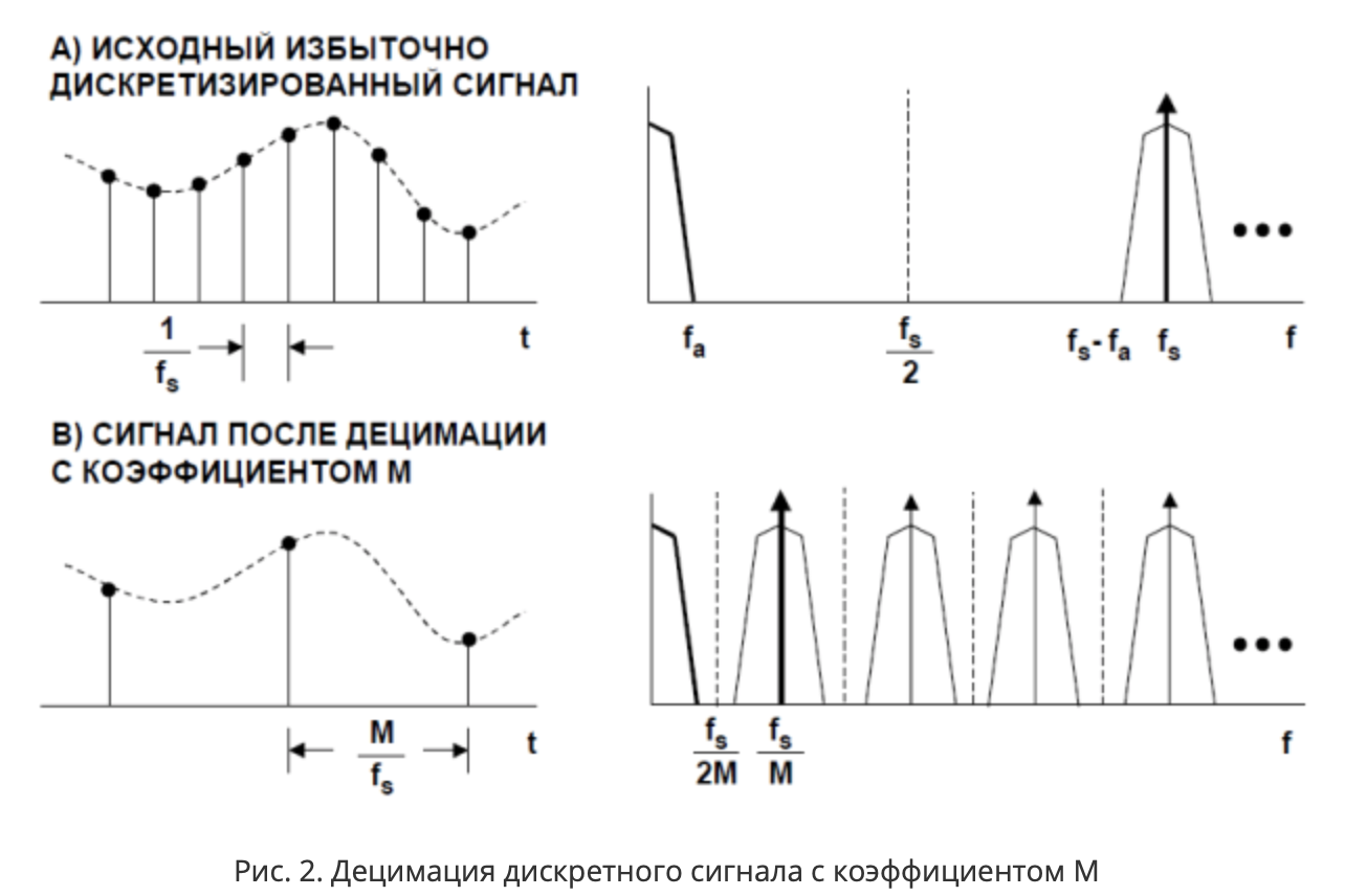
For FS = 32kHz, the Nyquist frequency will be 16kHz. In this case, the useful signal is unlikely to go beyond the band fa = 20Hz (very few people can change the direction of movement more often 20 times per second). In total, the sampling frequency is much higher than the frequency required for storing the information contained in the fa band (40 Hz, 400 times higher), that is, the useful signal is over-sampled. The band between the fa and fs-fa frequencies does not contain any useful information. You can reduce the sampling rate (in the diagram this is done with the coefficient M, [7]), after thinning out the sequence of samples (samples). This process is called decimation .
According to the specification for the MPU-9250, accelerometers are equipped with a sigma-delta ADC. Schemes based on it consume minimal power. It should be noted that the bandwidth of these converters is very narrow, does not exceed the audio range [Easyelectronics], but for a standard quadcopter more is not needed. They consist of two blocks: modulator and digital low-pass decimation filter.
Fair Excerpt from Wiki:
If the original signal does not contain frequencies higher than the Nyquist frequency of the decimated signal, then the spectrum of the received (decimated) signal coincides with the low-frequency part of the spectrum of the original signal. The sampling rate corresponding to the new sample sequence is N times lower than the sampling rate of the original signal.
If the source signal contains frequencies that are higher than the Nyquist frequency of the decimated signal, then aliasing (spectral overlap) will occur during the decimation.
Thus, to save the spectrum, it is necessary to remove frequencies from the original signal that are higher than the Nyquist frequency of the decimated signal before decimation. The specification for the MPU-9250 does not have much information about the characteristics of DLPF, but you can find research enthusiasts [9].
frequency range in which the sensor detects motion and provides a valid output. In some specifications, the frequency response of the sensor is given - the dependence of the electrical output signal of the accelerometer on external mechanical influences with a fixed amplitude but different frequencies. Within the passband, the non-uniformity of the frequency response does not exceed the given one. In the case of applying a digital low-pass filter, the choice of bandwidth just allows you to change the cutoff frequency, inevitably affecting the speed of the sensor response to changes in position in space. The cut-off frequency must be less than half the digitization rate (ODR), also called the Nyquist frequency.
For MPU-9250 accelerometers, the bandwidth limit is determined so that within the range the spectral density of the signal differs from the peak (at 0 Hz) by no more than –3 dB. This level roughly corresponds to a drop in half of the spectral density (or 70.7% of the peak spectral amplitude). Let me remind you that for energy values (power, energy, energy density), proportional to the squares of the field strengths, the ratio expressed in decibels
Bottom line: the signals passed through the low-pass filter are less noisy, they have better resolution, but with less bandwidth. Therefore, specifying the resolution in the specification without reference to the bandwidth does not make sense.
In the specification for the MPU-9250, there is no resolution information in principle, for the BMI088, the resolution is represented by the digital resolution (LSB) and sensitivity. ”
The resolution for each bandwidth can be estimated from peak noise The rms noise level at the output is related to the spectral density specified in the specification (or rather, the root of it) and the equivalent noise bandwidth (equivalent noise bandwidth, ENBW, equivalent bandwidth of the equivalent system that has a rectangular frequency response and the same and the variance at the output, when acting on the inputs of white noise systems):
  it turns out
  . At the same time, the specification specifies the full mean square noise.
 The discrepancy is significant. Unfortunately, it is indicated only for one band, and for the BMI088 accelerometer only PSD is indicated in the specification. So we will use what we have. Cross factor take 4. Now the most interesting. Attitude
 will give an approximate order of effective bits in a given measurement range, which is decently less than the 16-bit resolution of the ADC.
Out of the need to store variables in the internal buffer for dividing the signal into different frequencies by the filter
. The lower the cutoff frequency of the filter, the less noise in the signal. But here you have to be careful, because at the same time the delay also grows. In addition, you can skip the useful signal [8].
And these are only the most basic parameters.
Where did it come from:
It is a little about the main blocks of the inertial module.
MEMS gyro
The MPU-9250 consists of three independent uniaxial vibration angular velocity sensors (MEMS gyroscopes), which respond to rotation around the X, Y, and Z axes. Two suspended masses oscillate in opposite axes. With the advent of angular velocity, the Coriolis effect causes a change in the direction of the vibration (
which is fixed by a capacitive sensor. The measured differential capacitive component is proportional to the displacement angle [Electronics Time]. The resulting signal is amplified, demodulated and filtered, resulting in a voltage proportional to the angular velocity of rotation. This signal is digitized using the built-in 16-bit ADC board. The sample rate can programmatically vary from 3.9 to 8000 samples per second (samples per second, SPS), and user-defined low-pass filters (LPF) provide a wide range of possible cut-off frequencies. A low-pass filter is needed, including to remove vibrations from the motors (usually above 20-25 Hz).Three-axis MEMS accelerometer
For each axis, it uses a separate test mass, which is displaced when acceleration occurs along this axis (fixed by capacitive sensors). The MPU-9250 architecture reduces susceptibility to temperature drift and variations in electrical parameters. When the device is located on a flat surface, it will measure 0g along the X- and Y-axes and + 1g along the Z-axis. The scale factor (scale factor) is calibrated at the factory and does not depend on the supply voltage. Each sensor is equipped with an individual sigma-delta ADC (consists of a modulator and a digital low-pass filter, for more details about the device in [Easyelectronics]), the output digital signal of which has an adjustable measurement range.
And immediately about the three-axis MEMS magnetometer
Based on high-precision Hall effect technology. It includes magnetic sensors that determine the earth's magnetic field strength along axes, a control circuit, a signal amplification circuit, and a computational circuit for processing signals from each sensor. Each ADC has a resolution of 16 bits, the measurement range
. To measure weak magnetic fields, either a unit in the SI microtesla system (μT) or gauss (Gs, GHS system) is used:, [Radiolotsman]). So what is LSB and how to calculate it? Mining instructions
Suppose our accelerometer is now working in the measurement range
, that is, the full range of possible values will be . The corresponding voltage values are digitized by a 16-bit ADC, which can split the entire interval as much as possible intosteps. The minimum increment that can be detected is just one step.. Here we must remember that the account is conducted from scratch, so that in fact the maximum measured value will be. That is, the larger the bits in the digital word ADC or DAC, the smaller the discrepancy will be. In this case, the sensitivity (sometimes called the scale factor, the sensitivity scale factor) of the sensor on a specific range will be determined as the ratio of the electrical output signal and the mechanical effect. Traditionally indicated for a signal frequency of 100 Hz and temperature For the MPU-9250, the sensitivity is steps for every g or (, ), for another IMU, BMI088 from Bosch Sensortec, the sensitivity of the gyroscope is calculated in the same way, and for the accelerometer it is used steps on each g. The FS options are taken out of the specification for gyroscopes and, in order not to get up twice, accelerometers.
I took FS for accelerometers also from the BMI088 documentation (see below).
Gyroscope, 16 bit  | Accelerometer, 16 bits | ||
|---|---|---|---|
| Range (FS) (dps) | LSB, (dps) | Range (FS), g | LSB mg |
 (Fs = 250) (Fs = 250) | 0,004 |  (Fs = 4) (Fs = 4) | 0.06 |
 (Fs = 500) (Fs = 500) | 0,008 |  (Fs = 6) (Fs = 6) | 0.09 |
 (Fs = 1000) (Fs = 1000) | 0,0015 |  (Fs = 8) (Fs = 8) | 0.12 |
 (Fs = 2000) (Fs = 2000) | 0.03 |  (Fs = 12) (Fs = 12) | 0.18 |
 (FS = 4000) (FS = 4000) | 0.06 |  (Fs = 16) (Fs = 16) | 0.24 |
 (Fs = 24) (Fs = 24) | 0.37 | ||
 (Fs = 32) (Fs = 32) | 0.48 | ||
 (Fs = 48) (Fs = 48) | 0.73 | ||
Everything seems to fall into place, you can go further. In some cases (below, for example, a clipping from the documentation for BMI088), a parameter such as Resolution (Resolution) is separately indicated.
In fact, it seems, it turns out that it should be LSB. But why then do we see one value instead of several ones tied to specific ranges? I had to expand the list of investigated sources in search of answers.
What is resolution?
The minimum value that the sensor reliably sees is extremely important when trying to strike a balance between price and performance. This is not an accuracy - a high-resolution sensor may not be particularly accurate, as well as a low-resolution sensor in certain areas may have sufficient accuracy. Unfortunately, LSB only defines a theoretical minimum distinguishable value, provided that we can use all 16 bits of the ADC. This resolution is in the digital world. In analog, some of the steps will be noisy and the number of effective bits will be less.
What are the characteristics of noise and where does it come from?
Noise sources can generally be broken down into electronic noise schemes that convert motion into a voltage signal (Johnson thermal noise, shot noise, pink 1 / f flicker noise, etc.), and thermal mechanical (Brownian, due to the presence of small moving parts) from the sensor itself. The characteristics of the latter will depend on the resonant frequency of the mechanical part of the system.
(natural frequency of oscillation of the sensor ).RMS value of noise in the entire spectral range - Total RMS (Root mean square) Noise
Noise levels can be determined in several ways. You can consider them in the time or frequency domain (after the Fourier transform). In the first case, the residual noise is taken as the rms value of the signals from the fixed sensor (in fact, this is the standard deviation for the sample at
) for a certain period of time: 
Accelerations or angular rotational speeds below the level of broadband noise will be indistinguishable - that’s the actual resolution. The rms value of the ac voltage or current (often referred to as effective or effective) is equal to the magnitude of the constant signal, which will produce the same work in an active (resistive) load during a period. This approach is most effective in estimating broadband noise where white noise dominates.
For white noise, the ratio of the amplitude (instantaneous peak value) to the root mean square with a probability of 99.9% is
Such an attitude is called the cross-factor (crest factor, cross ratio). You can choose the probability of 95.5% - the cross factor will be equal to 4. In fact, noise signals behave not so well and can produce peaks that increase the cross factor up to 10 times. Some specifications may contain values.
or the multiplier itself. In the narrow low-frequency band of 0.1–10 Hz, the flicker noise “1 / f” plays the main role, for estimation of which the value of the peak-to-peak noise signal is used.
Spectral density
Sometimes it is more convenient to consider a signal in the frequency domain, where its description is called a spectrum (dependence of amplitude and phase on frequency). One of the possible noise characteristics in the specifications is called power spectral density of noise (PSD), noise spectral density, noise noise density, or simply noise density ). Describes the noise power distribution over a range of frequencies. Regardless of the representation of the electrical signal through the current or voltage, the instantaneous power dissipated in the load can be normalized (R = 1 Ohm) and expressed as
Average power dissipated by a signal over a period of time 


can be written as ![$ x (t) = \ frac {a_0} {2} + \ frac {1} {2} \ sum_ {n = 1} ^ {\ infty} [(a_n - ib_n) e ^ {in \ omega t} + (a_n + ib_n) e ^ {- in \ omega t}] = \ sum_ {n = - \ infty} ^ {\ infty} c_n e ^ {in \ omega t}, $](https://habrastorage.org/getpro/habr/formulas/4e4/4a8/4e1/4e44a84e1a254371ce9dda29bac81378.svg)
, In general, these coefficients can be represented as follows: 

and on frequency. Power spectral density periodic signal gives the distribution of signal power over the frequency range: 
The average normalized power of the actual signal will be 
tends to infinity, the sequence of pulses turns into a separate pulse , the number of spectral lines tends to infinity, the spectrum graph turns into a smooth frequency spectrum For this limiting case, you can define a pair of Fourier integral transforms 

- Fourier-image. The power spectral density of a random signal is determined through the limit

Since we assume that the average for the white noise of the sensors in a stationary state is zero (
), then the square of the rms value is equal to the variance and represents the total power in the normalized load: 

We look in the specification - there, in fact, under the name of the spectral density is indicated the square root of it with the corresponding dimension
or That is, the RMS value of the noise without specifying the frequency band on which it was considered (Bandwidth) is meaningless. A little more about the choice of bandwidth
At the output of the MEMS sensor, we receive signals of different frequencies. It is assumed that we have in advance some idea of the processes we are measuring. For example, when determining the acceleration vector of a drone, the noise is the vibration of the apparatus. Separate them from the desired signal by using a low-pass filter, which cuts off all frequencies above that (for example, 200 Hz). The MPU-9250 provides the ability to adjust the cut-off frequency of the low-pass filter using the parameter with the magic name DLPFCFG. It stands for Digital Low Pass Filter Configuration. Further, in the specification, here and there, no less mysterious type expressions (DLPFCFG = 2, 92Hz) surfaced, but after decoding, I had to go into another document, “Register Map and Descriptions”. It shows which sets of bits in which registers need to be written to achieve the desired effects:
By omitting the technical details of the configuration, we can say the following. This sensor provides custom filtering of readings not only for accelerometers, gyros, but also for temperature sensors. For each, there are a total of 7 to 10 modes characterized by such concepts as Bandwidth in Hz, delay in ms, sampling frequency (Fs) in kHz.
The column “Noise density” was added to the accelerometer filter mode table in
, and the “Bandwidth” column is supplemented with the value of “3dB”. It did not get any easier, so let's go straight through the list.
The legacy of ancient Rome
Sample rate + decimation
-ADC = data update rate (digital output data rate, ODR)With the sampling rate (the same sampling frequency), everything is clear - this is the number of points of a continuous signal taken per second when it is sampled by ADC. Measured in hertz.

In order for the sample to get a value close to the peak signal amplitude, it is important to take the sampling frequency at least 10 times the frequency of the useful signal. The MPU-9250 offers three options: Fs = 32kHz, 8kHz, 1kHz.
But this absolutely does not mean that the signal at the output of the accelerometer or gyroscope appears with the same period.
If you take the same drones, everything rests on the struggle to reduce energy consumption, increase the speed of calculations and reduce the noise of the output data. You can lower the update rate at the output, allowing the internal algorithms to integrate the input information over a period of time. The RMS will decrease, but the bandwidth will also decrease (the sensor can detect only those processes whose frequency will be less than 50% of the data update rate).
It is better to immediately recall the Kotelnikov theorem . It promises that when sampling an analog signal, you can avoid data loss (that is, restore the signal without distortion) if the frequency of the useful signal is no more than half the sampling rate, also called the Nyquist frequency . In practice, a classic anti-aliasing filter (a low-pass filter that reduces the contribution of side frequency components in the output signal to negligible levels - GOST R 8.714-2010) in most cases requires a difference of at least 2.5 times [Siemens].
For FS = 32kHz, the Nyquist frequency will be 16kHz. In this case, the useful signal is unlikely to go beyond the band fa = 20Hz (very few people can change the direction of movement more often 20 times per second). In total, the sampling frequency is much higher than the frequency required for storing the information contained in the fa band (40 Hz, 400 times higher), that is, the useful signal is over-sampled. The band between the fa and fs-fa frequencies does not contain any useful information. You can reduce the sampling rate (in the diagram this is done with the coefficient M, [7]), after thinning out the sequence of samples (samples). This process is called decimation .
According to the specification for the MPU-9250, accelerometers are equipped with a sigma-delta ADC. Schemes based on it consume minimal power. It should be noted that the bandwidth of these converters is very narrow, does not exceed the audio range [Easyelectronics], but for a standard quadcopter more is not needed. They consist of two blocks:
modulator and digital low-pass decimation filter. Why combine a low pass filter and decimation?
Fair Excerpt from Wiki:
If the original signal does not contain frequencies higher than the Nyquist frequency of the decimated signal, then the spectrum of the received (decimated) signal coincides with the low-frequency part of the spectrum of the original signal. The sampling rate corresponding to the new sample sequence is N times lower than the sampling rate of the original signal.
If the source signal contains frequencies that are higher than the Nyquist frequency of the decimated signal, then aliasing (spectral overlap) will occur during the decimation.
Thus, to save the spectrum, it is necessary to remove frequencies from the original signal that are higher than the Nyquist frequency of the decimated signal before decimation. The specification for the MPU-9250 does not have much information about the characteristics of DLPF, but you can find research enthusiasts [9].
Bandwidth, also known as frequency response
frequency range in which the sensor detects motion and provides a valid output. In some specifications, the frequency response of the sensor is given - the dependence of the electrical output signal of the accelerometer on external mechanical influences with a fixed amplitude but different frequencies. Within the passband, the non-uniformity of the frequency response does not exceed the given one. In the case of applying a digital low-pass filter, the choice of bandwidth just allows you to change the cutoff frequency, inevitably affecting the speed of the sensor response to changes in position in space. The cut-off frequency must be less than half the digitization rate (ODR), also called the Nyquist frequency.
For MPU-9250 accelerometers, the bandwidth limit is determined so that within the range the spectral density of the signal differs from the peak (at 0 Hz) by no more than –3 dB. This level roughly corresponds to a drop in half of the spectral density (or 70.7% of the peak spectral amplitude). Let me remind you that for energy values (power, energy, energy density), proportional to the squares of the field strengths, the ratio expressed in decibels

Bottom line: the signals passed through the low-pass filter are less noisy, they have better resolution, but with less bandwidth. Therefore, specifying the resolution in the specification without reference to the bandwidth does not make sense.
Back to resolution
In the specification for the MPU-9250, there is no resolution information in principle, for the BMI088, the resolution is represented by the digital resolution (LSB) and sensitivity. ”
The resolution for each bandwidth can be estimated from peak noise
The rms noise level at the output is related to the spectral density specified in the specification (or rather, the root of it) and the equivalent noise bandwidth (equivalent noise bandwidth, ENBW, equivalent bandwidth of the equivalent system that has a rectangular frequency response and the same and the variance at the output, when acting on the inputs of white noise systems): 


it turns out . At the same time, the specification specifies the full mean square noise.The discrepancy is significant. Unfortunately, it is indicated only for one band, and for the BMI088 accelerometer only PSD is indicated in the specification. So we will use what we have. Cross factor take 4. Now the most interesting. Attitude will give an approximate order of effective bits in a given measurement range, which is decently less than the 16-bit resolution of the ADC.| MPU-9250 | BMI088 | ||||
|---|---|---|---|---|---|
| Gyroscope | |||||
 |  | ||||
 |  | ||||
 |  |  | |  | |
| 523 | 0.41 | 1.6 | |||
| 250 | 0.2 | 0.8 | 230 | 0.27 | 1.1 |
| 184 | 0.17 | 0.69 | 116 | 0.19 | 0.76 |
| 92 | 0.12 | 0.49 | 64 | 0.14 | 0.57 |
| 41 | 0.08 | 0.32 | 47 | 0.12 | 0.49 |
| 20 | 0.06 | 0.23 | 32 | 0.1 | 0.4 |
| ten | 0.04 | 0.16 | 23 | 0.09 | 0.34 |
| five | 0.03 | 0.11 | 12 | 0.06 | 0.25 |
| Accelerometer | |||||
 |  | ||||
 |  | ||||
|  |  | |  |  |
| 218.1 | 5.6 | 22 | 280 | 3.4 | 14 |
| 99 | 3.8 | 15 | 145 | 2.4 | ten |
| 44.8 | 2.5 | ten | 80 | 1.8 | 7 |
| 21.2 | 1.7 | 7 | 40 | 1.3 | five |
| 10.2 | 1.2 | 4.9 | 20 | 0.9 | four |
| 5.05 | 0.9 | 3.4 | ten | 0.6 | 2.6 |
| 420 | 7.8 | 31 | five | 0.5 | 1.8 |
| 1046 | 12.3 | 49 | |||
Delay (ms), or where the delay comes from
Out of the need to store variables in the internal buffer for dividing the signal into different frequencies by the filter
. The lower the cutoff frequency of the filter, the less noise in the signal. But here you have to be careful, because at the same time the delay also grows. In addition, you can skip the useful signal [8].
| MPU-9250 | BMI088 | ||
|---|---|---|---|
| Gyroscope, 16 bit | |||
| Range (FS) (dps) | Resolution, bits (BW = 92Hz) | Range (FS) (dps) | Resolution, bit (BW = 64Hz) |
| eight | ||
| 9 | | 9 |
| ten | | ten |
| eleven | | eleven |
| 12 | | 12 |
| Accelerometer | |||
| Range (FS), g | Resolution, bit  | Range (FS), g | Resolution (X, Y), bits  |
| 6 | | eight |
| 7 | | 9 |
| eight | | ten |
| 9 | | eleven |
And these are only the most basic parameters.
Where did it come from:
- The most enjoyable document from Freescale Semiconductor is "How Many Bits are Enough?"
- [EE] - "Resolution vs Accuracy vs Sensitivity Cutting Through the Confusion"
- [Electronics Time] - “MEMS Motion Sensors from STMicroelectronics: Accelerometers and Gyros”
- [LSB] - “An ADC and DAC Least Significant Bit (LSB)”
- [Measurement Computing] - “TechTip: Accuracy, Precision, Resolution, and Sensitivity”
- [KIT] - “Analog Devices Accelerometers - device and application”
- [Easyelectronics] - “Sigma Delta ADC”
- [Radiolotsman] - “Magnetometers: principle of operation, error compensation”
- [SO] - “Noise Measurement”
- [Mide] - "Accelerometer Specifications: Deciphering an Accelerometer's Datasheet"
- [CiberLeninka] - Delta-Sigma ADC Filter
- [SciEd] - "Features of the implementation of digital filtering with changing the sampling rate"
- [MPU6050] - “Using the MPU6050's DLPF”
- [MPU9250_DLPF] - MPU9250 Gyro Noise DLPF work investigation
- Understanding Sensor Resolution Specifications
- Siemens Digital Signal Processing
- MEMS motion sensors from STMicroelectronics
- [TMWorld] - "Evaluating inertial measurement units"
- [Sklyar] - Sklyar B. Digital communication. Theoretical foundations and practical application.