Deep Learning: Transfer learning and fine tuning of deep convolutional neural networks
- Transfer
In a previous article in the Deep Learning series, you learned about comparing frameworks for symbolic deep learning. This article will focus on deep tuning of convolutional neural networks to increase the average accuracy and efficiency of the classification of medical images.

1. Comparison of frameworks for symbolic deep learning .
2. Transfer learning and fine tuning of deep convolutional neural networks .
3. The combination of a deep convolutional neural network with a recurrent neural network .
Note: further the narration will be conducted on behalf of the author.
A common cause of vision loss is diabetic retinopathy (DR), an eye disease in diabetes. Examination of patients using fluorescence angiography can potentially reduce the risk of blindness. Existing research trends show that deep convolutional neural networks (GNSS) are very effective for automatic analysis of large sets of images and for identifying distinguishing features by which images can be divided into different categories with virtually no errors. GSNS training rarely happens from scratch due to the lack of predefined sets with a sufficient number of images related to a certain area. Since it takes 2–3 weeks to train modern GNSS, the Berkley Vision and Learning Center (BVLC) has released final milestones for GNSS. In this publication, we use a pre-trained network: GoogLeNet. GoogLeNet is trained on a large set of natural ImageNet images. We transfer the recognized ImageNet weights as initials for the network, then set up a pre-trained, universal network for recognizing fluorescence angiography images of the eyes and improving the accuracy of DR prediction.
At the moment, extensive work has already been done on the development of algorithms and techniques for image processing to explicitly highlight the distinguishing features characteristic of patients with DR. The following universal workflow is used in the standard image classification:
Oliver Faust and his colleagues provide a very detailed analysis of models that use explicit highlighting of the hallmarks of DR. Vuyosevich and colleagues created a binary classifier based on a data set of 55 patients, explicitly highlighting the individual distinguishing features of lesions. Some authors used morphological image processing techniques to extract the hallmarks of blood vessels and bleeding, and then trained the support vector machine on a dataset of 331 images. Other experts report 90% accuracy and 90% sensitivity in the binary classification task on a dataset of 140 images.
Nevertheless, all these processes are associated with a significant investment of time and effort. To further improve the accuracy of predictions, huge amounts of labeled data are required. Image processing and distinguishing features in image data sets is a very complex and lengthy process. Therefore, we decided to automate image processing and the stage of distinguishing distinguishing features using GNSS.
Expertise is required to highlight distinguishing features in images. Selection functions in the GNSS automatically form images for certain areas without using any processing features of the distinguishing features. Thanks to this process, GSNs are suitable for image analysis:

Layers C - convolutions, layers S - pools and samples
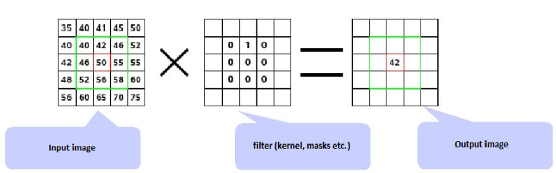
Convolution . Convolutional layers consist of a rectangular network of neurons. The weights are the same for each neuron in the convolutional layer. The weight of the convolutional layer determines the convolution filter.
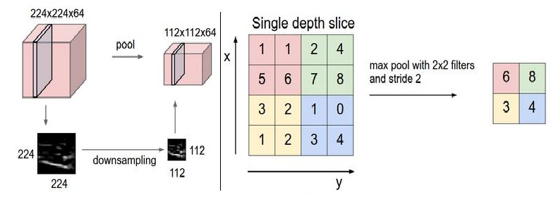
The survey . Pooling layer takes small rectangular blocks from a convolutional layer and performs subsampling to make one output from this block.
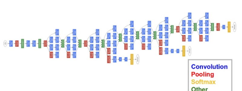
In this publication, we use the GoogLeNet GNSS developed by Google. Neural Network GoogLeNet won the ImageNet contest in 2014, setting a record for the best one-time results. The reasons for choosing this model are the depth of work and the economical use of architecture resources.
In practice, the training of entire GSNSs is usually not performed from scratch with arbitrary initialization. The reason is that it is usually not possible to find a dataset of a sufficient size required for a network of the desired depth. Instead, most of the time, pre-training of the GOOS takes place on a very large data set, and then the weights of the trained GOOS are used either as initialization or as highlighting the hallmarks for a specific task.
Fine tuning. Learning transfer strategies depend on various factors, but two are most important: the size of the new data set and its similarity to the original data set. Considering that the nature of the GNSS operation is more universal in the early layers and becomes more closely related to a specific data set in the subsequent layers, four main scenarios can be distinguished:
Fine-tuning the GNSS . Solving the issue of predicting DR, we act according to scenario IV. We fine-tune the scales of a pre-trained GSNS, continuing the reverse distribution. You can either fine-tune all layers of the GNSS, or leave some of the earlier layers unchanged (to avoid over-fitting) and configure only the high-level part of the network. This is due to the fact that the early layers of the GNSS contain more universal functions (for example, determining the edges or colors) that are useful for many tasks, and the later layers of the GNSS are already oriented to the classes of the DR data set.
Limitations of transfer learning. Because we use a pre-trained network, our choice of model architecture is somewhat limited. For example, we cannot arbitrarily remove convolutional layers from a pre-trained model. Nevertheless, due to the joint use of the parameters, it is possible to easily launch a pre-trained network for images of different spatial sizes. This is most obvious in the case of convolutional and sample layers, because their redirection function does not depend on the spatial size of the input data. In the case of fully connected layers, this principle is preserved, since fully connected layers can be converted into a convolutional layer.
Learning speed. We use a reduced training speed for GSNS weights that are fine-tuned, based on the fact that the quality of the scales of pre-trained GNSSs is relatively high. This data should not be distorted too quickly or too much, therefore both the learning speed and the drop in speed should be relatively low.
Data supplement. One of the disadvantages of irregular neural networks is their excessive flexibility: they are equally well trained in recognizing both details of clothing and interference, which increases the likelihood of overfitting. We apply Tikhonov regularization (or L2-regularization) to avoid this. However, even after that there was a significant performance gap between learning and checking DR images, which indicates an overfitting in the fine-tuning process. To eliminate this effect, we use data padding for the DR image dataset.
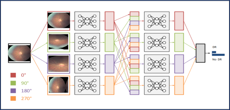
There are many ways to complement data, for example, flipping horizontally, randomly cropping, changing colors. Since the color information of these images is very important, we only use the rotation of the images at different angles: 0, 90, 180 and 270 degrees.
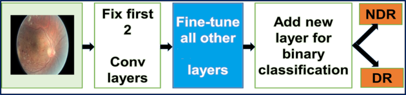
Replacing the input layer of a pre-trained GoogLeNet network with DR images. We fine-tune all layers except the top two pre-trained layers containing universal weights.
Fine-tuning GoogLeNet.The GoogLeNet we used was originally trained on the ImageNet dataset. The ImageNet dataset contains about 1 million natural images and 1000 tags / categories. Our tagged DR dataset contains about 30,000 images from the area in question and four tags / categories. Therefore, this DR dataset is not enough to train a complex network like GoogLeNet: we will use weights from the GoogLeNet network trained on ImageNet. We fine-tune all layers except the top two pre-trained layers containing universal weights. The initial loss3 / classifier classification layer outputs predictions for 1000 classes. We are replacing it with a new binary layer.
Thanks to fine-tuning, it is possible to apply advanced models of GNSS in new areas where it would be impossible to use them differently due to lack of data or time and cost limitations. This approach allows to achieve a significant increase in the average accuracy and efficiency of the classification of medical images.
If you see an inaccuracy in the translation, please report this in private messages.
Series of articles "Deep Learning"
1. Comparison of frameworks for symbolic deep learning .
2. Transfer learning and fine tuning of deep convolutional neural networks .
3. The combination of a deep convolutional neural network with a recurrent neural network .
Note: further the narration will be conducted on behalf of the author.
Introduction
A common cause of vision loss is diabetic retinopathy (DR), an eye disease in diabetes. Examination of patients using fluorescence angiography can potentially reduce the risk of blindness. Existing research trends show that deep convolutional neural networks (GNSS) are very effective for automatic analysis of large sets of images and for identifying distinguishing features by which images can be divided into different categories with virtually no errors. GSNS training rarely happens from scratch due to the lack of predefined sets with a sufficient number of images related to a certain area. Since it takes 2–3 weeks to train modern GNSS, the Berkley Vision and Learning Center (BVLC) has released final milestones for GNSS. In this publication, we use a pre-trained network: GoogLeNet. GoogLeNet is trained on a large set of natural ImageNet images. We transfer the recognized ImageNet weights as initials for the network, then set up a pre-trained, universal network for recognizing fluorescence angiography images of the eyes and improving the accuracy of DR prediction.
Using explicit highlighting to predict diabetic retinopathy
At the moment, extensive work has already been done on the development of algorithms and techniques for image processing to explicitly highlight the distinguishing features characteristic of patients with DR. The following universal workflow is used in the standard image classification:
- Image pre-processing techniques to remove noise and increase contrast.
- The technique of distinguishing distinguishing features.
- Classification.
- Prediction.
Oliver Faust and his colleagues provide a very detailed analysis of models that use explicit highlighting of the hallmarks of DR. Vuyosevich and colleagues created a binary classifier based on a data set of 55 patients, explicitly highlighting the individual distinguishing features of lesions. Some authors used morphological image processing techniques to extract the hallmarks of blood vessels and bleeding, and then trained the support vector machine on a dataset of 331 images. Other experts report 90% accuracy and 90% sensitivity in the binary classification task on a dataset of 140 images.
Nevertheless, all these processes are associated with a significant investment of time and effort. To further improve the accuracy of predictions, huge amounts of labeled data are required. Image processing and distinguishing features in image data sets is a very complex and lengthy process. Therefore, we decided to automate image processing and the stage of distinguishing distinguishing features using GNSS.
Deep convolutional neural network (GNSS)
Expertise is required to highlight distinguishing features in images. Selection functions in the GNSS automatically form images for certain areas without using any processing features of the distinguishing features. Thanks to this process, GSNs are suitable for image analysis:
- GNSS train networks with many layers.
- Multiple layers work together to form an improved feature space.
- The initial layers study the primary features (color, edges, etc.).
- Further layers study higher-order features (according to the input data set).
- Finally, the characteristics of the final layer are served in the classification layers.
Layers C - convolutions, layers S - pools and samples
Convolution . Convolutional layers consist of a rectangular network of neurons. The weights are the same for each neuron in the convolutional layer. The weight of the convolutional layer determines the convolution filter.
The survey . Pooling layer takes small rectangular blocks from a convolutional layer and performs subsampling to make one output from this block.
In this publication, we use the GoogLeNet GNSS developed by Google. Neural Network GoogLeNet won the ImageNet contest in 2014, setting a record for the best one-time results. The reasons for choosing this model are the depth of work and the economical use of architecture resources.
Transfer learning and fine tuning of deep convolutional neural networks
In practice, the training of entire GSNSs is usually not performed from scratch with arbitrary initialization. The reason is that it is usually not possible to find a dataset of a sufficient size required for a network of the desired depth. Instead, most of the time, pre-training of the GOOS takes place on a very large data set, and then the weights of the trained GOOS are used either as initialization or as highlighting the hallmarks for a specific task.
Fine tuning. Learning transfer strategies depend on various factors, but two are most important: the size of the new data set and its similarity to the original data set. Considering that the nature of the GNSS operation is more universal in the early layers and becomes more closely related to a specific data set in the subsequent layers, four main scenarios can be distinguished:
- The new dataset is smaller and similar in content to the original dataset. If the amount of data is small, then it makes no sense to fine-tune the GSNS due to overfitting. Since the data are similar to the original, it can be assumed that the distinctive features in the GOOS will be relevant for this data set. Therefore, the optimal solution is to train a linear classifier as a hallmark of the SNA.
- The new data set is relatively large and similar in content to the original data set. Since we have more data, you don’t have to worry about overfitting if we try to fine-tune the entire network.
- The new data set is smaller and significantly different in content from the original data set. Since the amount of data is small, only a linear classifier will be sufficient. Since the data are significantly different, it is better to train the classifier not from the top of the network, which contains more specific data. Instead, it’s better to train the classifier by activating it on earlier layers of the network.
- The new data set is relatively large and significantly different in content from the original data set. Since the data set is very large, you can afford to train the entire GSNS from scratch. Nevertheless, in practice it is often still more profitable to use it to initialize weights from a pre-trained model. In this case, we will have enough data to fine-tune the entire network.
Fine-tuning the GNSS . Solving the issue of predicting DR, we act according to scenario IV. We fine-tune the scales of a pre-trained GSNS, continuing the reverse distribution. You can either fine-tune all layers of the GNSS, or leave some of the earlier layers unchanged (to avoid over-fitting) and configure only the high-level part of the network. This is due to the fact that the early layers of the GNSS contain more universal functions (for example, determining the edges or colors) that are useful for many tasks, and the later layers of the GNSS are already oriented to the classes of the DR data set.
Limitations of transfer learning. Because we use a pre-trained network, our choice of model architecture is somewhat limited. For example, we cannot arbitrarily remove convolutional layers from a pre-trained model. Nevertheless, due to the joint use of the parameters, it is possible to easily launch a pre-trained network for images of different spatial sizes. This is most obvious in the case of convolutional and sample layers, because their redirection function does not depend on the spatial size of the input data. In the case of fully connected layers, this principle is preserved, since fully connected layers can be converted into a convolutional layer.
Learning speed. We use a reduced training speed for GSNS weights that are fine-tuned, based on the fact that the quality of the scales of pre-trained GNSSs is relatively high. This data should not be distorted too quickly or too much, therefore both the learning speed and the drop in speed should be relatively low.
Data supplement. One of the disadvantages of irregular neural networks is their excessive flexibility: they are equally well trained in recognizing both details of clothing and interference, which increases the likelihood of overfitting. We apply Tikhonov regularization (or L2-regularization) to avoid this. However, even after that there was a significant performance gap between learning and checking DR images, which indicates an overfitting in the fine-tuning process. To eliminate this effect, we use data padding for the DR image dataset.
There are many ways to complement data, for example, flipping horizontally, randomly cropping, changing colors. Since the color information of these images is very important, we only use the rotation of the images at different angles: 0, 90, 180 and 270 degrees.
Replacing the input layer of a pre-trained GoogLeNet network with DR images. We fine-tune all layers except the top two pre-trained layers containing universal weights.
Fine-tuning GoogLeNet.The GoogLeNet we used was originally trained on the ImageNet dataset. The ImageNet dataset contains about 1 million natural images and 1000 tags / categories. Our tagged DR dataset contains about 30,000 images from the area in question and four tags / categories. Therefore, this DR dataset is not enough to train a complex network like GoogLeNet: we will use weights from the GoogLeNet network trained on ImageNet. We fine-tune all layers except the top two pre-trained layers containing universal weights. The initial loss3 / classifier classification layer outputs predictions for 1000 classes. We are replacing it with a new binary layer.
Conclusion
Thanks to fine-tuning, it is possible to apply advanced models of GNSS in new areas where it would be impossible to use them differently due to lack of data or time and cost limitations. This approach allows to achieve a significant increase in the average accuracy and efficiency of the classification of medical images.
If you see an inaccuracy in the translation, please report this in private messages.