How to reduce the number of measurements and benefit from it
 At first I wanted to write honestly and in detail about the methods of reducing the dimensionality of data - PCA , ICA , NMF , dump a bunch of formulas and say what an important role SVD plays in this whole zoo. Then I realized that I would get a text similar to clippings from the opuses from Mathgen , so the number of formulas was minimized, but I left the most favorite code and pictures in full.
 I also thought about writing about auto encoders. In R, as you know, the trouble is with neural network libraries: either slow , or buggy , or primitive. This is understandable, because without full support for the GPU (and this is a huge minus R compared to Python), working with any kind of complex neural networks - and especially with Deep Learning - is almost pointless (although there is a promising developing MXNet project ). Also of interest is the relatively fresh h2o framework , whose authors are advised by the notorious Trevor Hastie , and Cisco, eBay and PayPal even use it to create their plans to enslave humanity. The framework is written in Java (yes, yes, and really loves RAM). Unfortunately, it also does not support working with the GPU, because It has a slightly different target audience, but it scales perfectly and provides an interface to R and Python (although fans of masochism can also use the web-interface hanging by default on localhost: 54321) .
So, if the question arose about the number of measurements in a data set, then this means that, well, let's say, there are quite a lot of them, which is why the use of machine learning algorithms becomes not very convenient. And sometimes part of the data is just informational noise, useless garbage. Therefore, it is advisable to remove unnecessary measurements by extracting from them as much as possible the most valuable. By the way, the inverse problem may arise - to add more dimensions, but simply more interesting and useful features. Dedicated components can also be useful for visualization purposes ( t-SNE is oriented to this, for example). Decomposition algorithms are interesting in and of themselves as machine learning methods without a teacher, which, you see, can sometimes even lead to the solution of a primary problem.
Matrix decompositions
In principle, to reduce the dimensionality of data with one or another efficiency, most of the methods of machine learning can be adapted - in fact, they are engaged in this, mapping one multidimensional space to another. For example, the results of PCA and K-means are in a sense equivalent. But usually you want to reduce the dimension of the data without much fuss with the search for model parameters. The most important of these methods, of course, is SVD . “Why SVD and not PCA?” You ask. Because SVD, firstly, in itself is a separate important technique in data analysis, and the matrices obtained as a result of decomposition have a completely meaningful interpretation from the point of view of machine learning; secondly, it can be used for PCA and with some reservations for NMF(as well as other matrix factorization methods); thirdly, SVD can be adapted to improve ICA performance . In addition, SVD does not have such uncomfortable properties as, for example, applicability only to square (decompositions of LU , Schur ) or square symmetric positive definite matrices ( Cholesky ), or only to matrices whose elements are non-negative ( NMF ). Naturally, one has to pay for universality - the singular decomposition is rather slow; therefore, when the matrices are too large, randomized algorithms are used .
The essence of SVD is simple - any matrix (real or complex) is represented as the product of three matrices:
X = UΣV* ,
where U is a unitary matrix of order m; Σ is a matrix of size mxn, on the main diagonal of which there are non-negative numbers called singular (elements outside the main diagonal are equal to zero - such matrices are sometimes called rectangular diagonal matrices); V * is a Hermitian conjugate to V matrix of order n. m columns of the matrix U and n columns of the matrix V are called the left and right singular vectors of the matrix X, respectively. For the problem of reducing the number of dimensions, it is the matrix Σ whose elements, being raised to the second degree, can be interpreted as the variance that each “puts” into the common cause component, and in decreasing order: σ 1 ≥ σ2 ≥ ... ≥ σ noise . Therefore, when choosing the number of components in SVD (as in PCA, by the way) they are guided precisely by the sum of the variances that the considered components give. In R, the singular decomposition operation is performed by the svd () function, which returns a list of three elements: the vector dc with singular values, the matrices u and v.
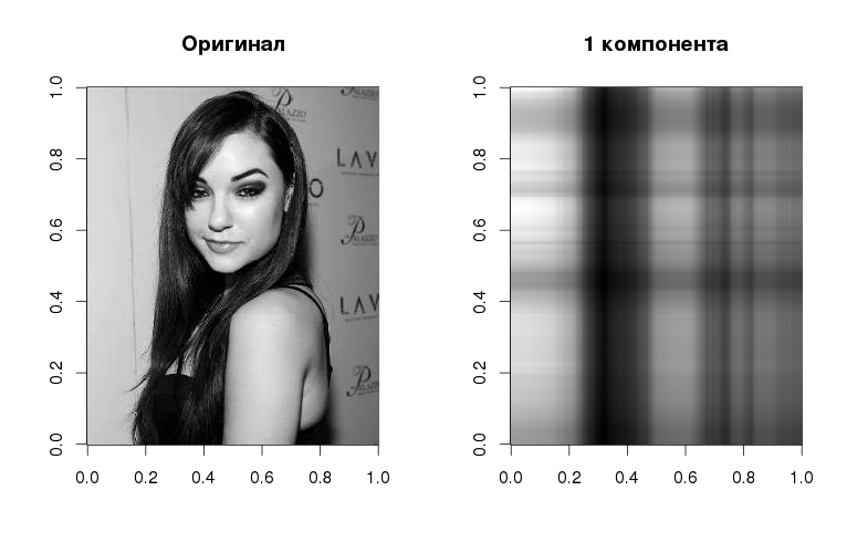
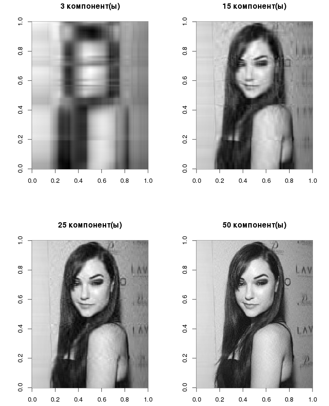
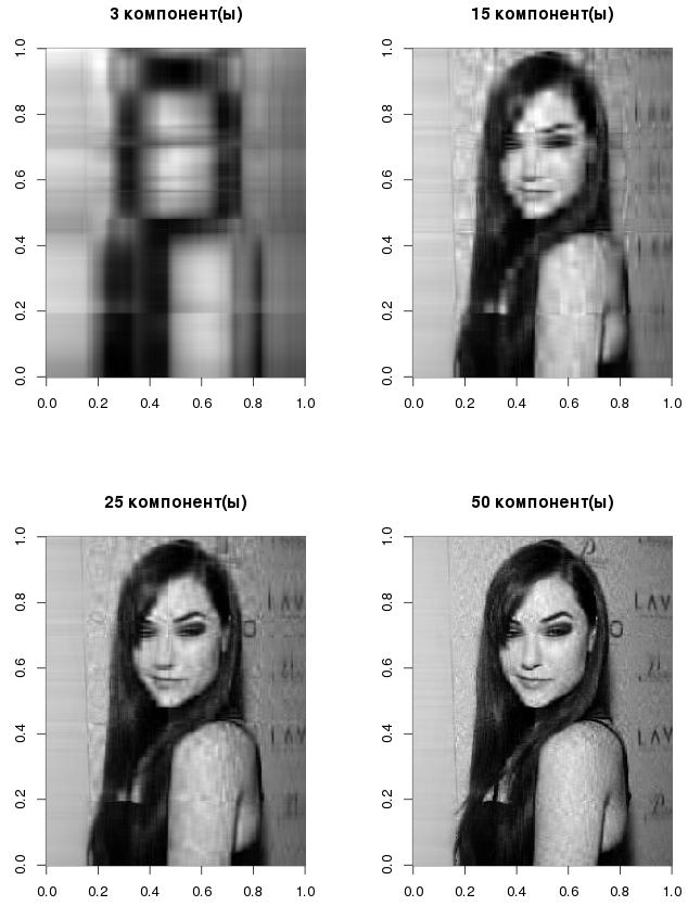
Yes, Sasha looks like this in gray halftones with only one component , but even here you can see the basic linearized structure - in accordance with the gradations in the original image. The component itself is obtained if we multiply the left singular vector by the corresponding singular value and the right singular vector. As the number of vectors increases, so does the quality of image reconstruction:
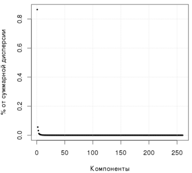
The following graph shows that the first component explains more than 80% of the variance:
R code, singular decomposition:
library(jpeg)
img <- readJPEG("source.jpg")
svd1 <- svd(img)
# Первая компонента
comp1 <- svd1$u[, 1] %*% t(svd1$v[, 1]) * svd1$d[1]
par(mfrow=c(1,2))
image(t(img)[,nrow(img):1], col=gray(0:255 / 255), main="Оригинал")
image(t(comp1)[,nrow(comp1):1], col=gray(0:255 / 255), main="1 компонента")
# Несколько компонент
par(mfrow=c(2,2))
for (i in c(3, 15, 25, 50)) {
  comp <- svd1$u[,1:i] %*% diag(svd1$d[1:i])%*% t(svd1$v[,1:i])
  image(t(comp)[,nrow(comp):1], col=gray(0:255 / 255), main=paste0(i," компонент(ы)"))
}
par(mfrow=c(1,1))
plot(svd1$d^2/sum(svd1$d^2),pch=19,xlab="Компоненты",ylab="% от суммарной дисперсии", cex=0.4)
grid()
What happens if we subtract the average values of each column from the original image, divide the resulting matrix into the square root of the number of columns in the original matrix, and then perform a singular decomposition? It turns out that the columns of the matrix V in the resulting decomposition will exactly correspond to the main components that are obtained with PCA (by the way, in R for PCA, you can use the prcomp () function)
> img2 <- apply(img, 2, function(x) x - mean(x)) / sqrt(ncol(img))
> svd2 <- svd(img2)
> pca2 <- prcomp(img2)
> svd2$v[1:2, 1:5]
            [,1]         [,2]          [,3]        [,4]        [,5]
[1,] 0.007482424 0.0013505222 -1.059040e-03 0.001079308 -0.01393537
[2,] 0.007787882 0.0009230722 -2.512017e-05 0.001324682 -0.01373691
> pca2$rotation[1:2, 1:5]
             PC1          PC2           PC3         PC4         PC5
[1,] 0.007482424 0.0013505222 -1.059040e-03 0.001079308 -0.01393537
[2,] 0.007787882 0.0009230722 -2.512017e-05 0.001324682 -0.01373691
Thus, when performing a singular decomposition of the normalized initial matrix, it is not difficult to isolate the main components. This is one way of calculating them; the second is based directly on finding the eigenvectors of the covariance matrix of the XX-th T .
Let us return to the question of choosing the number of principal components. The captain’s rule is this: the larger the components, the more variance they describe. Andrew Ng , for example, advises focusing on> 90% variance. Other researchers claim that this number may be 50%. Even the so-called parallel analysis of Horn was invented , which is based on a Monte Carlo simulation. In r for this and packagethere is. A very simple approach is to use scree plot : on the graph, you need to look for the "elbow" and discard all the components that form the gentle part of this "elbow". In the figure below, I would say 6 components should be taken into account:

In general, as you can see. the question is well worked out. It is also believed that the PCA is applicable only to normally distributed data, but the Wiki does not agree with this, and SVD / PCA can be used with data of any distribution, but, of course, not always efficiently (which is revealed empirically).
Another interesting expansion is the factorization of non-negative matrices , which, as the name implies, is used to decompose non-negative matrices into non-negative matrices:
X = WH .
In general, such a problem does not have an exact solution (unlike SVD), and numerical algorithms are used for its calculation. The problem can be formulated in terms of quadratic programming - and in this sense it will be close toThe SVM . In the problem of reducing the dimension of space, the following is important: if the matrix X has the dimension mxn, then the matrices W and H respectively have the dimensions mxk and kxn, and choosing k is much smaller than m and n themselves, we can significantly reduce this initial dimension. They like to use NMF for text data analysis , where non-negative matrices are in good agreement with the nature of the data, but in general the spectrum of application of the technique is not inferior to PCA. The decomposition of the first picture in R gives the following result:
Code for R, NMF:
library(NMF)
par(mfrow=c(2,2))
for (i in c(3, 15, 25, 50)) {
  m.nmf <- nmf(img, i)
  W <- m.nmf@fit@W
  H <- m.nmf@fit@H
  X <- W%*%H
  image(t(X)[,nrow(X):1], col=gray(0:255 / 255), main=paste0(i," компонент(ы)"))
}
If you need something more exotic
There is a method that was originally developed to decompose a signal with additive components - I'm talking about ICA . At the same time, the hypothesis is accepted that these components have an abnormal distribution, and their sources are independent. The simplest example is a party , where many voices are mixed, and the task is to isolate each sound signal from each source. Two approaches are usually used to search for independent components: 1) with minimization of mutual information based on the Kullback-Leibler divergence ; 2) with maximization of “non-Gaussianity” (here measures such as the excess coefficient and negentropy are used ).
In the picture below - a simple example where two sine waves are mixed, then they are also distinguished using ICA.

Code for R, ICA:
x <- seq(0, 2*pi, length.out=5000)
y1 <- sin(x)
y2 <- sin(10*x+pi)
S <- cbind(y1, y2)
A <- matrix(c(1/3, 1/2, 2, 1/4), 2, 2)
y <- S %*% A
library(fastICA)
IC <- fastICA(y, 2)
par(mfcol = c(2, 3))
plot(x, y1, type="l", col="blue", pch=19, cex=0.1, xlab="", ylab="", main="Исходные сигналы")
plot(x, y2, type="l", col="green", pch=19, cex=0.1, xlab = "", ylab = "")
plot(x, y[,1], type="l", col="red", pch=19, cex=0.5, xlab = "", ylab = "", main="Смешанные сигналы")
plot(x, y[,2], type="l", col="red", pch=19, cex=0.5, xlab = "", ylab = "")
plot(x, IC$S[,1], type="l", col="blue", pch=19, cex=0.5, xlab = "", ylab = "", main="ICA")
plot(x, IC$S[,2], type="l", col="green", pch=19, cex=0.5, xlab = "", ylab = "")
What does the ICA have to do with the task of reducing data dimension? Let's try to present the data - regardless of their nature - as a mixture of components, then it will be possible to divide this mixture into the number of “signals” that suits us. There is no special criterion, as is the case with PCA, for the choice of the number of components - it is selected experimentally.
The last experimental in this review is auto - encoders , which are a special class of neural networks configured in such a way that the response at the output of the auto - encoder is as close as possible to the input signal. With all the power and flexibility of neural networks, we also get a lot of problems associated with finding the optimal parameters: the number of hidden layers and neurons in them, activation functions ( sigmoid , tanh, ReLu ,), the learning algorithm and its parameters, regularization methods ( L1, L2 , dropout ). If you train an auto encoder on noisy data so that the network recovers it, you get denoising autoencoder . Preset auto-encoders can also be “docked” in the form of cascades for pre-training deep networks without a teacher.
In its simplest representation, an auto encoder can be modeled as a multilayer perceptron , in which the number of neurons in the output layer is equal to the number of inputs. From the figure below it is clear that by choosing an intermediate hidden layer of small dimension, we thereby “compress” the original data.

Actually, in the h2o package , which I mentioned above, such an auto-associator is present, so we will use it. At first I wanted to set an example with gestures , but I quickly became convinced that you won’t get

The data is presented in the form of .csv files (train.csv and test.csv), there are quite a lot of them, so in the future I will work with 10% of the data from train.csv to simplify; the column with labels will be used for visualization purposes only. But before we figure out what can be done using an auto-encoder, let's see what the first three components give us when decomposing PCA, ICA, NMF:
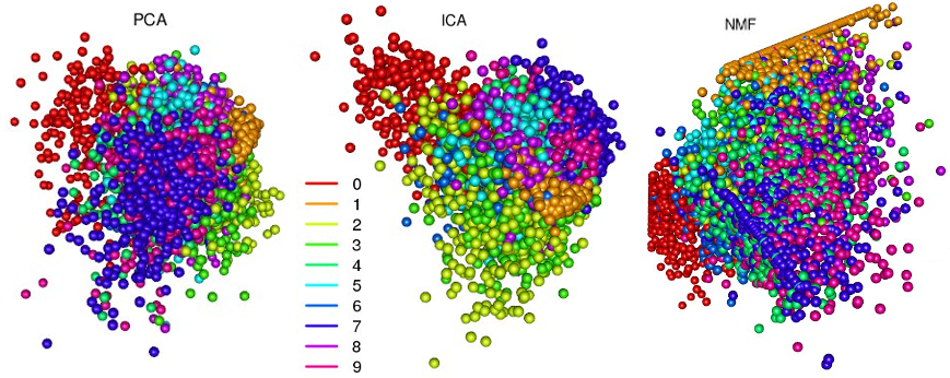
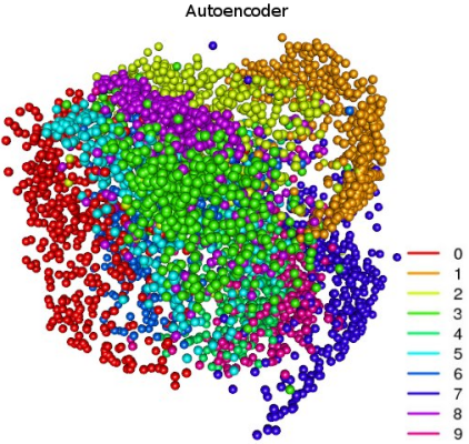
All three methods did a good job of clustering - in the image more or less clearly visible groups that smoothly transition into each other. These transitions are borderline cases when numbers are especially difficult to recognize. In the figure with PCA clusters, it is very clearly visible how the principal component method solves an important problem - decorrelates variables: clusters “0” and “1” are maximally spaced. The “unusual” pattern with NMF is connected precisely with the fact that the method works only with non-negative matrices. But such a separation of sets can be obtained using an auto-encoder:
Code on R, h2o auto encoder:
train <- read.csv("train.csv")
label <- data$label
train$label <- NULL
train <- train / max(train)
# Подготовка выборки для обучения
library(caret)
tri <- createDataPartition(label, p=0.1)$Resample1
train <- train[tri, ]
label <- label[tri]
# Запуска кластера h2o
library(h2o)
h2o.init(nthreads=4, max_mem_size='14G')
train.h2o <- as.h2o(train)
# Обучение автоэнкодера и выделение фич
m.deep <- h2o.deeplearning(x=1:ncol(train.h2o),
                           training_frame=train.h2o,
                           activation="Tanh",
                           hidden=c(150, 25, 3, 25, 150),
                           epochs=600,
                           export_weights_and_biases=T,
                           ignore_const_cols=F,
                           autoencoder=T)
deep.fea <- as.data.frame(h2o.deepfeatures(m.deep, train.h2o, layer=3))
library(rgl)
palette(rainbow(length(unique(labels))))
plot3d(deep.fea[, 1], deep.fea[, 2], deep.fea[, 3], col=label+1, type="s",
       size=1, box=F, axes=F, xlab="", ylab="", zlab="", main="AEC")
Here, clusters are more clearly defined and spaced apart in space. The network has a fairly simple architecture with 5 hidden layers and a small number of neurons; in the third hidden layer there are only 3 neurons, and the features from there are just depicted above. Some more interesting pictures:
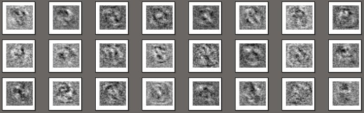
R code, visualization of the weights of the first hidden layer:
W <- as.data.frame(h2o.weights(m.deep, 1))
pdf("fea.pdf")
for (i in 1:(nrow(W))){
  x <- matrix(as.numeric(W[i, ]), ncol=sqrt(ncol(W)))
  image(x, axes=F, col=gray(0:255 / 255))
}
dev.off()
In fact, these are just images of neuron weights: each picture is associated with a separate neuron and represents a filter that selects information specific to a given neuron. Here is a comparison of the scales of the output layer:

The aforementioned auto-encoder can be easily turned into a denoising autoencoder. Since such an auto-encoder needs to submit distorted images to the input, it’s enough to place a dropout layer before the first hidden layer . Thanks to it, with some probability, neurons will be in the “off” state, which a) will introduce distortions into the processed image; b) will serve as a kind of regularization in training.
Another interesting application of the auto encoder is the determination of anomalies in the data on image reconstruction error. In general, if the data from the training set is not fed to the input of the auto-encoder, then, of course, the reconstruction error of each image from the new sample will be higher than that of the training set, but more or less of the same order. In the presence of anomalies, this error will be tens or even hundreds of times more.
Conclusion
Of course, it would be wrong to write that some compression method is better or worse than others: each has its own specifics and scope; a lot depends on the nature of the data itself. Not the last role here is played by the speed of the algorithm. Of the above, the fastest turned out to be SVD / PCA, then ICA, NMF go in order, and the auto-encoder completes the series. It is especially difficult to work with an auto-associator - not least due to the non-triviality in the selection of parameters.