FPGA Digital Filtering - Part 1
- Tutorial
Hello!
I have long wanted to start a series of articles devoted to digital signal processing on FPGAs, but for various reasons I could not begin to do this. Fortunately, a little free time appeared at the disposal, so I will periodically publish materials that reflect various aspects related to DSP on FPGAs.

In these articles, I will try to minimize the theoretical description of various algorithms and devote most of the material to the practical subtleties that I personally and my colleagues and friends have encountered in one way or another related to FPGA development. I hope this series of articles will benefit both novice engineers and experienced developers.
In the first part we will consider the simplest CIC filter . CIC - "cascaded integral-comb", in Russian - a cascade integral-comb filter of the IIR type (with infinite impulse response). The class of such filters is widely used in tasks where work is required at several data rates. CIC filters are actively used for decimation and interpolation, that is, to lower and increase the sampling frequency. The CIC filter itself is nothing more than a low-pass filter (low-pass filter). That is, such a filter passes the lower frequencies of the spectrum, cutting off the upper ones behind the cutoff frequency. The frequency response of the filter is constructed according to the law ~ sin (x) / x . The main advantage of CIC filters is that they do not require multiplication operations at all (unlike other types of filters, for example, FIR).
From the name you can guess that the CIC filter is based on two basic units: an integrator and a comb filter (differentiator). The integrating element (int) is an ordinary first-order IIR filter, made as the simplest battery. The comb filter (comb) is a first-order FIR filter.
Between the integrator and comb filter is often made enhance knot or lower sampling frequencies integer times - R .
The formulas for the transfer and amplitude-frequency characteristics are given below:

In more detail with all the mathematical calculations about all aspects of decimation and interpolation, you can read in other sources, which I will give links to at the end of the article.
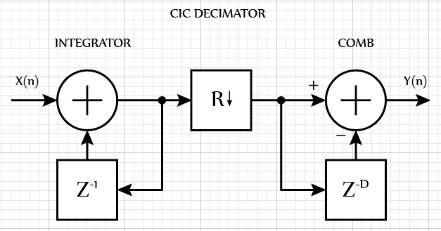
If a CIC filter is used to lower the sampling rate, then it is called a decimator. In this case, the integrator is the first link, then the sampling rate is lowered, and finally, the differentiating filter link goes.
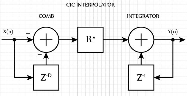
If a CIC filter is used to increase the sampling rate, then it is called an interpolator. In this case, the differentiating element is in the first place, then the sampling frequency is increased and, finally, there is an integrating filter link.
Depending on the delay of the input signal in the differentiating element, it is possible to obtain various frequency characteristics of the filter. It is known that as the delay parameter D increases, the number of “zeros” of the amplitude-frequency characteristic (AFC) of the filter increases.
Note that for a bunch of integrator and comb filter (CIC filter) with increasing parameter D in the differentiating section, the zeros of the frequency response shift to the center - the filter cutoff frequency Fc = 2 pi / D changes .
The cascade connection of an integrator and a comb filter without decimation and interpolation operations is called a moving average filter. The level of the first side lobe of such a filter is only -13 dB, which is small enough for serious DSP tasks.
Due to the linearity of the mathematical operations occurring in the CIC filter, it is possible to cascade several filters in a row. This gives a proportional decrease in the level of the side lobes, but also increases the obstruction of the main lobe of the spectrum (by the spectrum I will often mean the frequency response of the filter). Thus, for N-Cascade connection of the same type of CIC filters is the multiplication of identical transfer characteristics. As a rule, integrator and comb filter sections are combined together by type. For example, at first N sections of the same type of integrators are put sequentially, then N sections of the same type of differentiating filters.
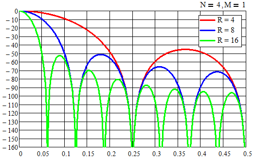
The following figure shows the frequency response of the filter for various parameters of the sampling coefficient R (calculation was done in MathCAD 14).
The frequency response of the CIC filter is fully equivalent to the frequency response of a FIR filter with a rectangular impulse response (TH). The total filter IC is defined as the convolution of all impulse characteristics of the cascades of the integrator and comb filter cascades. With the growth of the order of the CIC filter, their IC is integrated an appropriate number of times. Thus, for a CIC filter of the first order, THEM is a rectangle, for a filter of second order THEM is an isosceles triangle, for third order THEM is a parabola, etc.
Unfortunately, an increase in the delay value D in the comb structure and an increase in the order of the filter N lead to an increase in the transmission coefficient. This in turn leads to an increase in bit depth at the filter output. In DSP tasks where CIC filters are used, you should always remember this and make sure that the transmitted signals do not go beyond the used bit grid. For example, the negative effect of the increase in bit depth is manifested in a significant increase in the used resources of the FPGA chip.
Interpolator: the use of limited accuracy does not affect the internal bit depth of the registers, only the last output stage is scaled. A significant increase in bit depth occurs in the integrator sections.
Decimator:The CIC filter decimator is very sensitive to the parameters D, R and N, on which the bit depth of the intermediate and output data depends. Both the differentiating link and the integrator affect the final bit depth of the output signal.
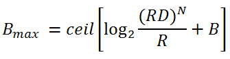
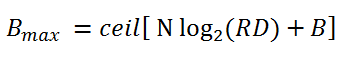
In these formulas: B is the bit depth of the input data, Bmax is the bit depth of the output data, R is the sampling rate, D is the delay parameter, N is the filter order (number of cascades).
Comment! The Hogenauer article describes the principles for choosing the bit depth for each stage of the decimator. When implementing their filters, Xilinx and Altera take into account the negative effect of increasing the filter capacity and fight this phenomenon with the methods described in the article.
Since my work is 99% related to Xilinx microcircuits, I will provide a description of the IP filter core for this vendor. But I dare to assure you that for Altera everything is almost the same.
In order to create a CIC filter, you need to go into the CORE Generator application and create a new project in which to indicate the type of FPGA used and various other settings that are not essential in this case.
CIC Compiler - Tab 1:

Component name name of the component (using the Latin letters az, numbers 0-9 and the symbol "_").
Filter Specification:
Sample Rate Change Specification:
Hardware Oversampling Specification: these parameters affect the output sample rate, the number of clock cycles required to process the data. The parallelism level inside the kernel and the amount of resources occupied also depend on these parameters.
* - the range depends on the general settings and the sampling rate R.
CIC Compiler - Tab 2:
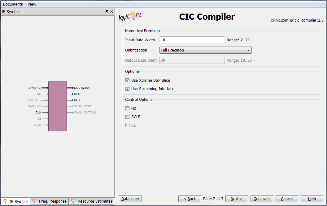
Numerical Precision:
Optional:
Control Options:
CIC Compiler - Tab 3:

Summary - this tab in the form of a list reflects the final filter settings (number of stages, frequency parameters, bit depth of input, output and intermediate data, delay in the filter, etc.).
The left side of the CIC Compiler window has three useful additional tabs:
After setting all the settings, click on the Generate button . As a result, after some time, the CORE Generator application will produce a whole set of files, of which we need the most basic:
If you work in the ISE Design Suite environment, the CORE Generator will automatically create the necessary files in the working directory. For other development tools (such as Modelsim or Aldec Active-HDL), you need to transfer the necessary files to the appropriate working directory.
Example 1: For modeling, the MATLAB program is a very convenient tool. For example, take a 4-order CIC filter model made on logic elements from the System Generator Toolbox from Xilinx. Decimation and interpolation are not used (CIC degenerates into a moving average filter with window 16). Filter parameters: R = 1, N = 4, D = 16. The following figure shows a model of one cascade in MATLAB.
Let us see what the impulse response looks like after each stage of the filter; for this, we apply a periodic unit impulse to the input of the system.
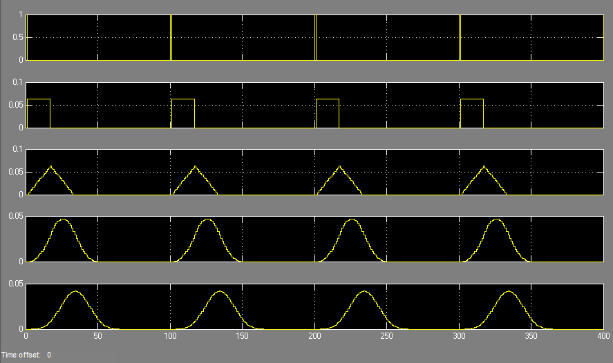
It can be seen that the signal at the output of the first link forms a rectangular pulse of duration = D, the output of the second link - a triangular signal of duration 2D, the output of the third link - a parabolic pulse, the output of the third - a cubic parabola. The result is fully consistent with theory.
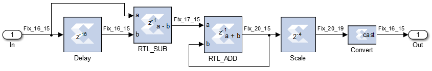
Example 2: The IP core of the CIC filter itself. Parameters: N = 3, R = 4, D = 1. The following figure shows the filter model.
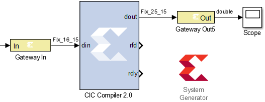
If a single pulse of several clock cycles (for example 32) is applied to the input of such a filter, then a parabolic signal is formed at the output, which resembles a THIR filter of a moving average.

Summary
I would like to summarize this. CIC filters are used in many tasks where it is necessary to change the sampling rate. CIC filters are used in systems operating at several multirate processing frequencies, for example, in audio technology to change the bit rate (from 44.1 kHz to 48 kHz and vice versa). CIC filters are used in communication systems for the implementation of DDC (digital down converter) and DUC (digital up converters). CIC Filter Example: AD6620 Digital Reception Chip from Analog Devices.
Implementing your own filter on FPGAs in HDL languages is often not required, and you can safely use ready-made kernels from vendors, or ready-made opensource projects. If you nevertheless need to implement your own CIC filter for the application, you need to remember the following principles.
CIC filters have a number of features:
Literature
To be continued...
I have long wanted to start a series of articles devoted to digital signal processing on FPGAs, but for various reasons I could not begin to do this. Fortunately, a little free time appeared at the disposal, so I will periodically publish materials that reflect various aspects related to DSP on FPGAs.
In these articles, I will try to minimize the theoretical description of various algorithms and devote most of the material to the practical subtleties that I personally and my colleagues and friends have encountered in one way or another related to FPGA development. I hope this series of articles will benefit both novice engineers and experienced developers.
Part 1: CIC Filter
In the first part we will consider the simplest CIC filter . CIC - "cascaded integral-comb", in Russian - a cascade integral-comb filter of the IIR type (with infinite impulse response). The class of such filters is widely used in tasks where work is required at several data rates. CIC filters are actively used for decimation and interpolation, that is, to lower and increase the sampling frequency. The CIC filter itself is nothing more than a low-pass filter (low-pass filter). That is, such a filter passes the lower frequencies of the spectrum, cutting off the upper ones behind the cutoff frequency. The frequency response of the filter is constructed according to the law ~ sin (x) / x . The main advantage of CIC filters is that they do not require multiplication operations at all (unlike other types of filters, for example, FIR).
Introduction
From the name you can guess that the CIC filter is based on two basic units: an integrator and a comb filter (differentiator). The integrating element (int) is an ordinary first-order IIR filter, made as the simplest battery. The comb filter (comb) is a first-order FIR filter.
Between the integrator and comb filter is often made enhance knot or lower sampling frequencies integer times - R .
- In the case of lowering the sampling frequency from the input sequence, each R-sample is selected, forming a thinned output sequence.
- In the case of increasing the sampling frequency between the samples of the input sequence, zeros are simply inserted, which are then smoothed in the integrating section, forming a sequence at an increased sampling frequency.
The formulas for the transfer and amplitude-frequency characteristics are given below:
In more detail with all the mathematical calculations about all aspects of decimation and interpolation, you can read in other sources, which I will give links to at the end of the article.
Decimator
If a CIC filter is used to lower the sampling rate, then it is called a decimator. In this case, the integrator is the first link, then the sampling rate is lowered, and finally, the differentiating filter link goes.
Interpolator
If a CIC filter is used to increase the sampling rate, then it is called an interpolator. In this case, the differentiating element is in the first place, then the sampling frequency is increased and, finally, there is an integrating filter link.
Depending on the delay of the input signal in the differentiating element, it is possible to obtain various frequency characteristics of the filter. It is known that as the delay parameter D increases, the number of “zeros” of the amplitude-frequency characteristic (AFC) of the filter increases.
Note that for a bunch of integrator and comb filter (CIC filter) with increasing parameter D in the differentiating section, the zeros of the frequency response shift to the center - the filter cutoff frequency Fc = 2 pi / D changes .
The cascade connection of an integrator and a comb filter without decimation and interpolation operations is called a moving average filter. The level of the first side lobe of such a filter is only -13 dB, which is small enough for serious DSP tasks.
Due to the linearity of the mathematical operations occurring in the CIC filter, it is possible to cascade several filters in a row. This gives a proportional decrease in the level of the side lobes, but also increases the obstruction of the main lobe of the spectrum (by the spectrum I will often mean the frequency response of the filter). Thus, for N-Cascade connection of the same type of CIC filters is the multiplication of identical transfer characteristics. As a rule, integrator and comb filter sections are combined together by type. For example, at first N sections of the same type of integrators are put sequentially, then N sections of the same type of differentiating filters.
The following figure shows the frequency response of the filter for various parameters of the sampling coefficient R (calculation was done in MathCAD 14).
The frequency response of the CIC filter is fully equivalent to the frequency response of a FIR filter with a rectangular impulse response (TH). The total filter IC is defined as the convolution of all impulse characteristics of the cascades of the integrator and comb filter cascades. With the growth of the order of the CIC filter, their IC is integrated an appropriate number of times. Thus, for a CIC filter of the first order, THEM is a rectangle, for a filter of second order THEM is an isosceles triangle, for third order THEM is a parabola, etc.
Bit depth increase
Unfortunately, an increase in the delay value D in the comb structure and an increase in the order of the filter N lead to an increase in the transmission coefficient. This in turn leads to an increase in bit depth at the filter output. In DSP tasks where CIC filters are used, you should always remember this and make sure that the transmitted signals do not go beyond the used bit grid. For example, the negative effect of the increase in bit depth is manifested in a significant increase in the used resources of the FPGA chip.
Interpolator: the use of limited accuracy does not affect the internal bit depth of the registers, only the last output stage is scaled. A significant increase in bit depth occurs in the integrator sections.
Decimator:The CIC filter decimator is very sensitive to the parameters D, R and N, on which the bit depth of the intermediate and output data depends. Both the differentiating link and the integrator affect the final bit depth of the output signal.
In these formulas: B is the bit depth of the input data, Bmax is the bit depth of the output data, R is the sampling rate, D is the delay parameter, N is the filter order (number of cascades).
Comment! The Hogenauer article describes the principles for choosing the bit depth for each stage of the decimator. When implementing their filters, Xilinx and Altera take into account the negative effect of increasing the filter capacity and fight this phenomenon with the methods described in the article.
Xilinx CIC Filter
Since my work is 99% related to Xilinx microcircuits, I will provide a description of the IP filter core for this vendor. But I dare to assure you that for Altera everything is almost the same.
In order to create a CIC filter, you need to go into the CORE Generator application and create a new project in which to indicate the type of FPGA used and various other settings that are not essential in this case.
CIC Compiler - Tab 1:
Component name name of the component (using the Latin letters az, numbers 0-9 and the symbol "_").
Filter Specification:
- Filter type - filter type: interpolating / decimating.
- Number of stages - the number of cascades of integrators and comb filters: 3-6.
- Differential delay - delay in the differential filter cells: 1-2.
- Number of channels - the number of independent channels: 1-16.
Sample Rate Change Specification:
- Fixed / Programmable - type of sampling coefficient R: constant / programmable.
- Fixed or Initial Rate - value of the sampling coefficient R: 4..8192.
- Minimum Rate - the minimum value of the sampling coefficient R: 4..8.
- Maximum Rate - the maximum value of the sampling coefficient R: 8..8192.
Hardware Oversampling Specification: these parameters affect the output sample rate, the number of clock cycles required to process the data. The parallelism level inside the kernel and the amount of resources occupied also depend on these parameters.
- Select format - select the frequency ratio of the filter: Frequency Specification / Sample period.
- Frequency Specification : The user sets the sampling rate and the frequency of data processing.
- Sample period - Clock specification: the user sets the ratio of the processing frequency to the clock frequency of the data.
- Input Sampling Frequency - * .
- Clock frequency - filter processing frequency: * .
- Input Sampling period - the ratio of the processing frequency to the frequency of the input clock signal: * .
* - the range depends on the general settings and the sampling rate R.
CIC Compiler - Tab 2:
Numerical Precision:
- Input Data Width - width of input data: 2..20.
- Quantization - rounding of output data: full accuracy / rounding of the bit grid.
- Output Data Width - the width of the output data, the range depends on the coefficients N, D and R (the maximum value is 48 bits).
Optional:
- Use Xtreme DSP Slice - use the built-in DSP blocks to implement the filter.
- Use Streaming Interface - use a stream interface for multi-channel filter implementation.
Control Options:
- ND - “New data”, an input signal that determines the data input to the filter input.
- SCLR - synchronous filter reset (a logical unit at this input performs a reset).
- CE - “Clock Enable”, filter clock enable signal.
CIC Compiler - Tab 3:
Summary - this tab in the form of a list reflects the final filter settings (number of stages, frequency parameters, bit depth of input, output and intermediate data, delay in the filter, etc.).
The left side of the CIC Compiler window has three useful additional tabs:
- IP-symbol is a schematic view of an IP block with active I / O ports.
- Freq. response - transfer characteristic of the CIC filter.
- Resource estimate - an estimation of occupied resources.
After setting all the settings, click on the Generate button . As a result, after some time, the CORE Generator application will produce a whole set of files, of which we need the most basic:
- * .VHD (or * .V ) - source file for modeling on VHDL or Verilog.
- * .VHO is a useless file, but from it you can take a description of the component and porting for insertion into the project.
- * .NGC - netlist file. Contains a description of the architecture of the IP core (the components used and the signal connections between them) for the selected FPGA chip.
- * .XCO - a log file in which all parameters and settings of the IP kernel are stored. Useful file when working with Xilinx ISE Design Suite .
If you work in the ISE Design Suite environment, the CORE Generator will automatically create the necessary files in the working directory. For other development tools (such as Modelsim or Aldec Active-HDL), you need to transfer the necessary files to the appropriate working directory.
CIC Filter in MATLAB
Example 1: For modeling, the MATLAB program is a very convenient tool. For example, take a 4-order CIC filter model made on logic elements from the System Generator Toolbox from Xilinx. Decimation and interpolation are not used (CIC degenerates into a moving average filter with window 16). Filter parameters: R = 1, N = 4, D = 16. The following figure shows a model of one cascade in MATLAB.
Let us see what the impulse response looks like after each stage of the filter; for this, we apply a periodic unit impulse to the input of the system.
It can be seen that the signal at the output of the first link forms a rectangular pulse of duration = D, the output of the second link - a triangular signal of duration 2D, the output of the third link - a parabolic pulse, the output of the third - a cubic parabola. The result is fully consistent with theory.
Example 2: The IP core of the CIC filter itself. Parameters: N = 3, R = 4, D = 1. The following figure shows the filter model.
If a single pulse of several clock cycles (for example 32) is applied to the input of such a filter, then a parabolic signal is formed at the output, which resembles a THIR filter of a moving average.
Summary
I would like to summarize this. CIC filters are used in many tasks where it is necessary to change the sampling rate. CIC filters are used in systems operating at several multirate processing frequencies, for example, in audio technology to change the bit rate (from 44.1 kHz to 48 kHz and vice versa). CIC filters are used in communication systems for the implementation of DDC (digital down converter) and DUC (digital up converters). CIC Filter Example: AD6620 Digital Reception Chip from Analog Devices.
Implementing your own filter on FPGAs in HDL languages is often not required, and you can safely use ready-made kernels from vendors, or ready-made opensource projects. If you nevertheless need to implement your own CIC filter for the application, you need to remember the following principles.
CIC filters have a number of features:
- Easy to implement and do not require multiplication operations.
- Decimation and interpolation on CIC filters is used everywhere to quickly change the sampling rate, both integer and fractional times.
- With increasing filter order N and delay D, the bit depth of the intermediate and output data increases.
- With an increase in the order of the filter N, the suppression of the side lobes increases and the unevenness of the main lobe of the frequency response increases.
- It is recommended to use filters of the order of no more than 6-8, as as the order increases, implementation becomes more complicated, the amount of resources occupied increases, and the frequency response of the filter also distortes within the bandwidth.
- With an increase in the delay parameter D of the comb filter, the filter cutoff frequency changes, but for practical purposes, in cascade connection, the parameter D <3.
- When decimation in R times significantly increases the bit depth at the output of the filter.
- During interpolation, the main contribution to the bit depth of the intermediate and output data is made only by integrating links.
- The frequency response of the CIC filter is equivalent to the frequency response of the FIR filter with a rectangular impulse response. The total filter IC is defined as the convolution of all impulse characteristics of the cascades of the integrator and comb filter cascades.
- When changing the frequency at the output of the filter in the FPGA, the clock enable signal is used, but the processing frequency is not changed.
- If the ratio “processing frequency / sampling frequency” >> 1, it is possible to reuse filter resources in the FPGA, thereby implementing processing with a minimum expenditure of crystal resources for a multi-channel system.
- In modern FPGAs, CIC filters are implemented on DSP blocks (Xilinx, Altera), but in the absence of free resources, implementation on logical cells (SLICEs) is possible.
- After the CIC filter, it is recommended to put a multiplier with a programmable gain (gain multiplier), which will adjust the signal level to the desired dynamic range
- CIC filters introduce distortion into the spectrum of the output signal, therefore, after the CIC filter, it is necessary to install a compensating FIR filter (the calculation procedure is presented in the Altera datasheet, MATLAB is required for calculation).
Literature
- E. Ifeachor, B. Jervis. Digitaal l SignProcessing: A Practical Approach (2nd Edition).
- Hogenauer, E. An economical class of digital filters for decimation and interpolation.
- Wikipedia CIC filter
- Altera CIC Filter Userguide
- Xilinx CIC Compiler DS613
- MATLAB CIC Filter
- DSPLIB - CIC Filters
- DSPLIB - CIC decimator and interpolator
- Verilog source code with explanations
- OpenCores project 1. Last name of the author is very interesting :)
- Opencores project 2
To be continued...