Disjoint sets and the mysterious Ackerman function
- Tutorial
 We are talking about a simple data structure - a system of disjoint sets . In short: disjoint sets are given (for example, connected components of a graph) and by two elements x and y you can: 1) find out if x and y are in the same set; 2) combine the sets containing x and y. The structure itself is very simple to implement and has been described many times in various places (for example, there is a good article on the Habré and in some other places) But this is one of those amazing algorithms, writing that costs nothing, but figuring out why it works effectively is not easy. I will try to present a relatively simple proof of the exact estimate for the operating time of this data structure, invented by Zeidel and Sharier in 2005 (it differs from the horror that many could see elsewhere). Of course, the structure itself will also be described, but along the way we’ll figure out what is the inverse Ackerman function, about which many know only that it is sooooo slowly growing.
Disjoint set system
Imagine that for some reason you had to support a set of n points with two queries: Union (x, y), which connects the points x and y with an edge, and IsConnected (x, y), which checks for points x and y, is it possible to pass from x to edges in y. How to solve such a problem?
First, it’s wise to think not about points, but about connected components. A connected component is a set of points at which from each point it is possible to go through edges to each other from the same set. Then Union (x, y) is just a union of components containing x and y (if they are not in the same component), and IsConnected (x, y) is a test to see if x and y are in the same component.
Secondly, it is convenient to choose in each component one particular highlightedthe top taken at random. Let Find (x) return the selected vertex from the component containing x. Using Find (x), the function IsConnected (x, y) is reduced to a simple comparison of Find (x) and Find (y): IsConnected (x, y) == (Find (x) == Find (y)). When two components are merged into one using Union, the selected vertex of one of the combined components ceases to be selected, because the selected vertex in one component is always one.
So, we abstracted from the original problem and reduced it to the solution of another, more general problem: we have a set of disjoint sets that can be combined using Union and in which there is a selected element obtained using Find. Formally, the structure can be described as follows: there is an initial set of singleton sets {x 1 }, {x 2 }, ..., {xn } with the following operations:
- Union (x, y) merges together sets containing elements x and y;
- Find (x) returns the selected element from the set containing the element x, i.e. if we take any y from the same set as x, then Find (y) = Find (x). Find is needed so that you can find out if two elements are in the same set.
Systems of disjoint sets, or rather their implementation, which will be discussed later, were invented at the dawn of computer science. This structure is sometimes called Union-Find. The systems of disjoint sets have many applications: they play a central role in the Kraskal algorithm for finding the minimum skeleton, are used in the construction of the so-called dominator tree (a natural thing in code analysis), they make it easy to follow the connected components in the graph, etc. I must say right away, even though this article contains a brief description of the implementation of the structure of disjoint sets itself, for a detailed discussion of the applications of these structures and implementation details, it is better to read the sources already cited on the hub and Maxim Ivanov. But it was always interesting for me to find out how that unusual estimate for the operating time of systems of disjoint sets is obtained, which is not even so easy to understand. So, the main goal of this article is the theoretical justification of the effectiveness of Union-Find structures.
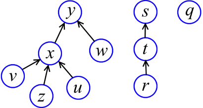
How to implement sets with Union-Find operations? The first thing that comes to mind is to store many sets of directed trees (see picture). Every tree is a multitude. The highlighted element of the set (the one that the Find function returns) is the root of the tree. To merge trees, you just need to attach the root of one tree to another.
Find (x) simply rises from x along the arrows until it reaches the root, and returns the root. But if you leave it as it is, it will easily turn out "bad" trees (such as a long "chain"), on which Find spends a lot of time. That is, “tall” trees do not need us.
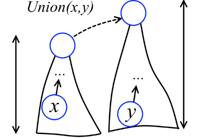
The height of the vertex x is the maximum path length from a leaf to x. For example, in the figure above, the height y - 2, x - 1, z - 0. With a little thought, you can equip each vertex with a height. We will call these heights ranks (looking ahead, I will say that these things are not called heights, as expected, because in the future the trees will be rebuilt and the ranks will no longer exactly correspond to the heights). Now when two trees are combined, the lower tree will cling to the higher one (see the figure below).
We realize it! We define element nodes as follows:
struct elem {
  elem *link; //указатель на родителя узла
  int rank;    //ранг узла
  double value; //какое-то хранящееся значение элемента
};
Initially, for each element x, x.link = 0 and x.rank = 0. You can already write a union function and a preliminary version of the Find function:
void Union(elem *x, elem *y)
{
  x = Find(x);
  y = Find(y);
  if (x != y) {
    if (x->rank == y->rank)
      y->rank++;
    else if (x->rank > y->rank)
      swap(x, y);
    x->link = y;
  }
}
elem *Find(elem *x) //первая плохая версия Find
{
  return x->link ? Find(x->link) : x;
}
Even such an implementation is already quite effective. To see this, we prove a couple of simple lemmas.
Lemma 1. In the Union-Find implementation with rank optimization, each tree with root x contains ≥2 x-> rank vertices.
Evidence. For trees consisting of one vertex x, x-> rank = 0 and it is clear that the statement of the lemma holds. Let Union combine trees with roots x and y for which the statement of the lemma is true, i.e. trees with roots x and y contain ≥2 x-> rank and ≥2 y-> rank vertices, respectively. A problem may arise if x joins y and the rank of y increases. But this only happens if x-> rank == y-> rank. Let r be the rank of y before the union. So the new tree with root y contains ≥2 x-> rank+ 2 r = 2 2 r = 2 r + 1 vertices. And this was required to prove.
Lemma 2. In Union-Find with rank optimization, the rank of each vertex x is equal to the height of the tree with root at x.
Evidence.When the algorithm is just getting started and all the sets are singleton, for each vertex x-> rank = 0, which is undoubtedly a height. Let Union combine two trees with roots x and y and let the heights of these trees be exactly equal to the corresponding ranks x-> rank and y-> rank. We show that even after the union, the ranks are equal to the heights. If x-> rank <y-> rank, then x will be hooked to y and, obviously, the height of the tree with the root y will not change; Union doesn’t really change y-> rank. The case x-> rank> y-> rank is similar. If x-> rank == y-> rank, then after attaching x to y, the height y will increase by one; and Union just increases y-> rank by one. Which was required.
It follows from Lemma 1 that the rank of any vertex cannot be greater than log n (we have all the logarithms in base 2), where n denotes the number of elements. And from Lemma 2 it follows that the height of any tree does not exceed log n. Therefore, each Find operation is performed in O (log n). Therefore, m Union-Find operations are performed in O (m log n).
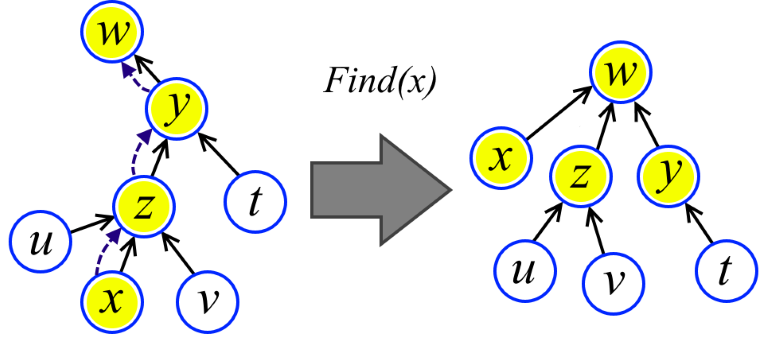
Is it even more efficient? The second optimization comes to the rescue. When performing an ascent in the Find procedure, we simply redirect all the vertices traversed to the root (see the figure). It certainly won’t get any worse. But it turns out to be much better.
elem * Find(elem *x)
{
  return x->link ? (x->link = Find(x->link)) : x;
}
So, we have a sequence of m operations Union and Find on n elements and we need to estimate how long it works. Could it be O (m log n)? Or O (m log log n)? Or is it O (m)?
It seems intuitively that an algorithm with a second optimization should be more efficient. And so it is, but to prove it is not so simple. Having analyzed a little, we can assume that the algorithm is linear, i.e. a sequence of m operations Union and Find shuffled in O (m). But no matter how you try, it will not be possible to prove this strictly, because it is not so. The first complete proof of the exact upper and lower bounds was given by Taryan in 1975 and this boundary was “almost” O (m), but, unfortunately, not O (m). Then followed works in which it was proved that in principle it is impossible to obtain O (m). Honestly, I could not figure it all out; even a counterexample showing that Union-Find is slower than for O (m) is quite difficult to understand. But fortunately, in 2005, Seidel and Sharir received a new relatively “understandable” proof of the upper bound. Their article is called "Top-down analysis of path compression." It is their result in a slightly simplified form that I will try to present here. Finding an “understandable” proof of the lower boundary can be considered an unresolved problem.
Is it so bad that we have not grown together with O (m)? Actually, all this is of purely theoretical interest, because the “almost” O (m) obtained by Taryan is indistinguishable from O (m) on all imaginable input data (it will soon become clear why). I must say right away that there will be no evidence that this will not be O (m) (I just don’t quite understand it myself), so it may seem that you can still a little and ... But you can’t. At least, despite some failed attempts, critical errors could not be found in the work of Taryan and a series of related works. The well-known attempt in the article “The Union-Find Problem is Linear”, according to the author himself, is erroneous, citation: “This paper has an error and has been retracted. It should simply be deleted from Citeseer. Baring that, I am submitting this “correction“. ”.
Stars, Stars, Stars
What kind of functions are those that give “almost” O (m)? Consider some function f such that f (n) <n for all n> 1, but f (n) tends to infinity. The function f grows slowly: its entire graph is under the graph of the function g (n) = n. We define the iteration operator * , which makes the super slow function f * from the slow function f :
f * (n) = min {k: f (f (... f (n))) <2, where f is taken k times}
That is, f * (n) shows how many times it is necessary to compress the number n by the operations f (n)> f (f (n))> f (f (f (n ()))> ... to get a constant of less than two.
A couple of examples to get comfortable. If f (n) = n-2, then f * (n) = [n / 2] (the integer part of the division by two). If f (n) = n / 2, then f* (n) = [log n] (the integer part of the binary logarithm). If f (n) = log n, then what is f * (n) = log * n? The log * n function is called the iterated logarithm . Slightly scribbling on paper, we can prove that log * n = O (log log n), log * n = O (log log log n) and generally log * n = O (log log ... log n) for any number logs. To imagine how slow the iterated logarithm is, just look at the value log * 2 65536 = 5.
In what follows, it will be shown that the execution time of m Union-Find operations can be estimated as O (m log *n) and, moreover, one can derive the estimates O (m log ** n), O (m log *** n), and so on, up to a certain limit function O (m α (m, n)) defined below. In general, I believe that for modern practical applications, O (m log log n) is almost indistinguishable from O (m). And O (m log * n) is generally indistinguishable from O (m), which is to say about O (m log ** n) and others. Now we can imagine why we are talking about “almost” O (m).
Grade O (m log * n)
Obtaining an estimate of O (m log * n) is an essential part of the proof. After that, an accurate estimate will be obtained almost immediately. To make it easier, we make one insignificant assumption: m ≥ n.
Without limiting the generality of reasoning, we assume that the Union operation always accepts the “roots” of sets, that is, Union is called like this: Union (Find (x), Find (y)). Then Union is executed in O (1). This restriction is all the more natural, because Union (x, y) first of all just calls Find (x) and Find (y). Therefore, in the analysis we will be interested only in Find operations.
We continue to simplify. Imagine that Find operations are not performed at all and the user somehow guesses where the roots of the sets are. A sequence of unions builds forest F (a forest is a lot of trees). By Lemma 2 in F, the rank of each vertex x is the height of the subtree with root at x. It follows that the rank of each vertex is less than the rank of the parent of this vertex. For us, this observation is important.
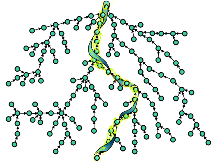
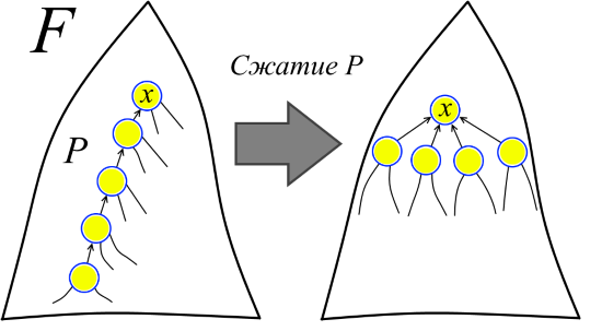
Let us return the sequence of Finds to the system. One can imagine that the first Find runs along some path in F and performs the operation of compressing the pathin F, at which each vertex of the path becomes the offspring of the vertex in the "head" of the path (see figure). Moreover, the head of the path is not necessarily the root of F. In other words, we agree that in a sense, all Union were executed in advance, and now on the forest F, the paths corresponding to Find are compressed in the normal course of the algorithm. Then the second Find runs along some path already in the modified forest (in the original forest F this path might not even exist at all) and again compresses the path. Etc.
It is important to note that after compression of the path, the ranks do not change. Therefore, we call ranks ranks, not heights, because in a modified forest, ranks may no longer correspond to heights.
Now we can clearly state what we are proving. There is a forest sequence F = F 1 , F2 , ..., F m and the sequence of contractions of the paths P 1 , P 2 , ..., P m in the forests F 1 , F 2 , ..., F m , respectively. The compression of the path P 1 in the forest F 1 receives the forest F 2 , the compression of the path P 2 in F 2 receives F 3 and so on. (Moreover, for example, the path P k might not yet exist in the forest F and appeared only after the paths P 1 , P 2 , ..., P k-1 were compressed ) It is necessary to estimate the sum of the path lengths P 1 , P 2, ..., P m (path length is the number of edges in the path). So we get an estimate for the execution time of m Find operations, because the length of the compressible path is just the number of vertex “relinking” operations in the corresponding Find.
Actually, we set out to prove an even more general statement than necessary, because not every sequence of path compressions corresponds to the sequence of Union-Find operations. But these nuances do not interest us.
So, there is a forest F and a sequence of path contractions in it in the sense that was attached to this above, i.e. there is a sequence of forests F = F 1 , F 2 , ..., F m and a sequence of contraction paths P 1 , P 2 , ..., P min them. Let T (m, n) denote the sum of the lengths of compressible paths P 1 , P 2 , ..., P m in the worst case, when the sum of the lengths P 1 , P 2 , ..., P m is maximal. The task is to estimate T (m, n). This is a purely combinatorial task, and all non-trivial evidence of Union-Find's effectiveness naturally reduces in one way or another to this construction.
Estimation of compressible path lengths
The first essentially nontrivial step in the discussion is the introduction of an additional parameter. The rank of the forest F is the maximum among the ranks of the vertices F. By T (m, n, r) we denote, similarly to T (m, n), the sum of the lengths of the compressible paths P 1 , P 2 , ..., P m in the worst case when the sum of the lengths P 1 , P 2 , ..., P m is maximum, and the source forest has a rank of no more than r. It is clear that T (m, n) = T (m, n, n), because the rank of any forest with n vertices is less than or equal to n. The parameter r is needed for the recursive reduction of the estimation problem for the forest F to the subtasks on the undergrowth F.
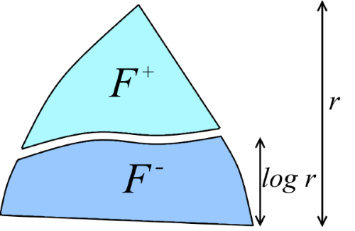
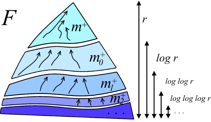
Denote d = log r. Divide the forest F into two disjoint forests F + and F -: The “upper forest” F + consists of peaks with a rank> d, and the “lower forest” F - consists of all other peaks (see figure). This partition was noticed even in the first evidence of Union-Find estimates in connection with the following fact: it turns out that the upper forest F + contains significantly fewer vertices than F - .
The main idea is to roughly estimate the lengths of the path compressions lying in F + (this can be done because F + is very small), and then recursively estimate the lengths of the path compressions in F - . That is, informally, our goal is to derive the recursion T (m, n, r) ≤ T (m, n, d) + (the lengths of paths not included in F -) We begin to move towards this goal by formalizing what means that F + is “very small”. Denote by | F '| the number of peaks in an arbitrary forest F '.
Lemma 3. Let F + be a forest consisting of vertices F of rank> d. Then | F + | <| F | / 2 d .
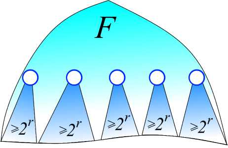
Evidence. We fix some t> d. Let us estimate how many vertices of rank t in F + . In F, by Lemma 2, the rank of a vertex is equal to the height of a tree with a root at a given vertex. Therefore, the parent of a vertex with a rank t necessarily has a rank> t. Thus, subtrees F with roots with rank t do not intersect (see the figure below). A tree with a root of rank t by Lemma 1 contains ≥2 t vertices. Therefore, in total there exists ≤n / 2 tvertices with rank t. Running t along d + 1, d + 2, ..., we see that the number of vertices in F + is bounded above by the infinite sum n / 2 d + 1 + n / 2 d + 2 + n / 2 d + 3 + ... By the geometric progression summation formula, we obtain that this sum is equal to n / 2 d . Which was required.
From here on, for brevity, we denote n + = | F + | and n - = | F - |.
The second non-trivial step in reasoning. We divide the set of paths P 1 , P 2 , ..., P m into three subsets (see the figure):
- P + - paths entirely contained in F + ;
- P - - paths entirely contained in F - ;
- P + - are paths having vertices from both F + and F - .

Each path from the set P + - is divided into two paths: the upper path in F + (white vertices in the figure below to the left) and the lower path in F - (green vertices in the figure below to the left). We just put the upper paths into the many P + paths . Denote by m + the number of paths in the set thus obtained, i.e. m + = | P + | + | P + - | (unlike the similar notation | F '| for forests, | P | denotes the number of paths in the set P, and not the total number of vertices in them). Denote m - = | P - |. Then:
T (m, n, r) ≤ T (m + , n + , r) + T (m -, n - , d) + (the sum of the lengths of the lower parts of the paths from P + - ).
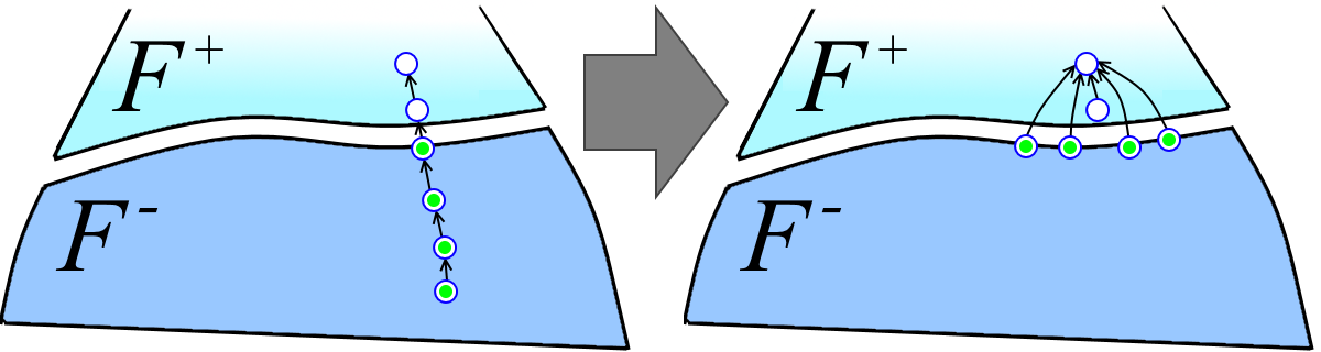
Let us estimate the sum of the lengths of the lower parts of the paths from P + - . Let P be the lower part of the path from P + - (green vertices in the figure above). All vertices in P except the head one had parents from F - before the linking (the head one necessarily has a parent from F + ), and after the linking they have a parent from F + (see the figure above). Therefore, each vertex from F - can participate in some lower part of the path from P + - as non-head only once. It turns out that the sum of the lengths of the lower parts of the paths from P + is less than or equal to | P + -| + n - (one for each head vertex, plus one for each vertex from F - ). Note that | P + - | ≤ m + . Therefore, the sum of the lengths of the lower parts of the paths from P + - does not exceed m + + n - .
An important note: in the discussion, it did not matter that the rank of F is less than or equal to d = log r; instead of log r, there could be any other value. If you get to this place, then congratulations, we just proved the central lemma.
The central lemma. Let F + - forest of peaks F with ranks> d, and F - - forest remaining vertices of F. The designations m +, m - , n + , n - are defined by analogy. Then the recursion is valid: T (m, n, r) ≤ T (m + , n + , r) + T (m - , n - , d) + m + + n - .
As already mentioned, since the F + forest is very small, the path lengths in it can be estimated using rough methods. Let's do it. Obviously, the compression of a path of length k in F + performs a k-1 vertex linking; that is, k-1 peak "rises" up the tree. The height F + does not exceed r and therefore each vertex can rise no more than r times. Therefore, m + path compressions perform at most rn+ relinks (ie “lifting” the peaks). From this we conclude that the sum of the lengths m + of the path contractions in F + is bounded above by the number rn + + m + (one for each vertex climb and one for the head of each path). By Lemma 3, we obtain rn + ≤ rn / 2 d = rn / 2 log r = n. As a result, we obtain T (m + , n + , r) ≤ n + m + . Using the central lemma, we derive the recursion:
T (m, n, r) ≤ T (m + , n + , r) + T (m - , n - , log r) + m + + n - ≤
≤ n + m + + T (m - , n, log r) + m + + n =
= 2n + 2m + + T (m - , n, log r).
Now, recursively, we continue to act in the same manner on forest F - in the same way as we did on forest F, i.e. just open the recursion:
T (m, n, r) ≤ (2n + 2m + ) + T (m - , n, log r)
≤ (2n + 2m + ) + (2n + 2m 0 + ) + T (m 0 - , n, log log r) ≤
≤ (2n + 2m + ) + (2n + 2m 0 + ) + (2n + 2m 1 + ) + T (m 1- , n, log log log r) ≤
≤ ...
Here m 0 + , m 1 + , ... are the values corresponding to m + at different levels of recursion. It is clear that m + + m 0 + + m 1 + + ... ≤ m (see the figure below). The recursion depth is the number of times that r must be prologged to get a constant. But this is log * r! As a result, we derive T (m, n, r) ≤ 2m + 2n log * r.
Ackerman's Inverse Final Solution
If we take a closer look at the findings, we can see that, in general, the value of log r played a role only in expanding the expression T (m + , n + , r) to obtain T (m + , n + , r) ≤ n + m + . This was achieved using Lemma 3 and a naive argument proving that T (m + , n + , r) ≤ rn + + m + . But in the previous section, we got a better estimate: T (m + , n + , r) ≤ 2m + + 2n + log * r. We redefine our main characters, "lowering" the forest F - : F +- a forest of peaks F with rank> the log * r, and F - - forest remaining vertices with rank the log ≤ * r. By analogy, we determine the parameters m + , m - , n + , n - .
By Lemma 3, we obtain n + <n / 2 log * r , i.e. the F + forest is still “small” compared to F - (at first it seemed to me even counterintuitive). In the previous section, we established that T (m + , n + , r) ≤ 2m + + 2n + log * r. Hence, given that 2 (n / 2 x) x ≤ n for any integer x ≥ 1, we derive T (m + , n + , r) ≤ 2m + + 2 (n / 2 log * r ) log * r ≤ 2m + + n. It is almost like the estimate T (m + , n + , r) ≤ n + m + obtained earlier! Using the central lemma, we obtain the recursion:
T (m, n, r) ≤ T (m + , n + , r) + T (m - , n - , log * r) + m + + n - .
Opening T (m + , n + , r) ≤ 2m + + n, we transform the recursion:
T (m, n, r) ≤ T (m + , n + , r) + T (m - , n - , log * r) + m + + n - ≤
≤ 2m + + n + T (m - , n - , log * r) + m + + n - ≤
≤ 3m + + 2n + T (m - , n, log * r).
Now we will reveal a couple of recursion levels:
T (m, n, r) ≤ (3m + + 2n) + T (m - , n, log * r)
≤ (3m + + 2n) + (3m 0 ++ 2n) + T (m 0 - , n, log * log * r) ≤
(3m + + 2n) + (3m 0 + + 2n) + (2m 1 + + 2n) + T (m 1 - , n , log * log * log * r) ≤
≤ ...
Here, as in the previous section, m 0 + , m 1 + , ... are the values corresponding to m + at different levels of recursion. It is clear that m + + m 0 + + m 1 + + ... ≤ m. The recursion depth is log** r. As a result, T (m, n, r) ≤ 3m + 2n log ** r. Very good mark. But can this focus be done once more using the just obtained estimate T (m, n, r) ≤ 3m + 2n log ** r? Yes!
Details I will omit this time. By “lowering” the forest F - to the rank of log ** r, we can again use Lemma 3 to obtain T (m + , n + , r) ≤ 3m + + n. This is almost like the just established estimate of T (m + , n + , r) ≤ 2m + + n. Then, using this estimate and the central lemma, we derive T (m, n, r) ≤ 4m + 2n log *** r.
We can continue further by “lowering” F -to rank log *** r. In general, having performed this procedure k times for any positive integer k, one can obtain the following estimate:
| T (m, n, r) ≤ km + 2n log ** ... * r, where the number of stars is k-1. |
It remains to optimize this recurrence relation. The more stars, the smaller the term 2n log ** ... * r, but the more km. Equilibrium is achieved at some k. But we will do it ruder: we turn the term n log ** ... * r into 2m. Before this final step, instead of r, we substitute everywhere n - the upper bound on the rank of the original forest F (although by Lemma 1 we could put r = log n, but not the point). We introduce the following function:
| α (m, n) = min {k: n log ** ... * n <2m, where the number of stars is k}. |
The function α (m, n) is called the function of the inverse to the Ackerman function . Let me remind you that we are only interested in the case m ≥ n. By definition of α (m, n), the expression n log ** ... * n, in which α (m, n) stars, is less than 2m. Actually, we introduced the function α (m, n) to obtain such an effect with a minimum of stars. Maybe this was not immediately noticeable, but we just proved that m Union-Find operations are performed in O (m α (m, n)).
Tadam!
A little bit about the inverse function of Ackerman
If you saw the inverse Ackerman function earlier, then most likely the definition was different (more incomprehensible), but giving in the end the same function asymptotically. The initial definition of Ackerman, which is used by Taryan, personally does not tell me anything about this function (in this case, for the area for which Ackerman himself introduced his function, the definition was natural). The definition proposed by Zeidel and Sharir (and just given) reveals the “secret meaning” of the reverse Ackerman. I would also add that, strictly speaking, “the function inverse to the Ackerman function” is an incorrect name, because α (m, n) is a function of two variables and it cannot be “inverse” to any function in any way. Therefore, it is sometimes said that α (m, n) is the pseudoinverse of Ackerman . I will not give the function of Ackerman.
Now a little bit of analysis. The maximum α (m, n) is achieved at m = n. Even very small deviations (e.g. m ≥ n log ***** n) make α (m, n) a constant. The function α (n, n) grows more slowly than log ** ... * n for any number of stars. By the way, the definition of α (n, n) looks similar to the definition of iteration:
α (n, n) = min {k: log ** ... * n <2, where the number of stars is k}.
Of course, this is not the limit and there are functions that grow even slower, for example log α (n, n). Another thing is surprising: α (m, n) arises in the analysis of such a natural algorithm. Even more surprisingly, there is evidence that it is impossible to improve the resulting estimate O (m α (m, n)).