Delivering Voice over the Mobile Network: Step 2 - Analog to Digital Conversion
In the first part of a series of articles, we examined the conversion of a human voice into an electrical signal. Now, it would seem, it's time to transmit this signal to the location of the interlocutor and start a conversation! That is exactly what they originally did. However, the more popular the service became and the greater the need to transmit a signal over long distances, the more clear it became that the analog signal was not suitable for this.
In order to ensure the transmission of information at any distance without loss of quality, we will need to make a second conversion from an Analog signal to a Digital one.
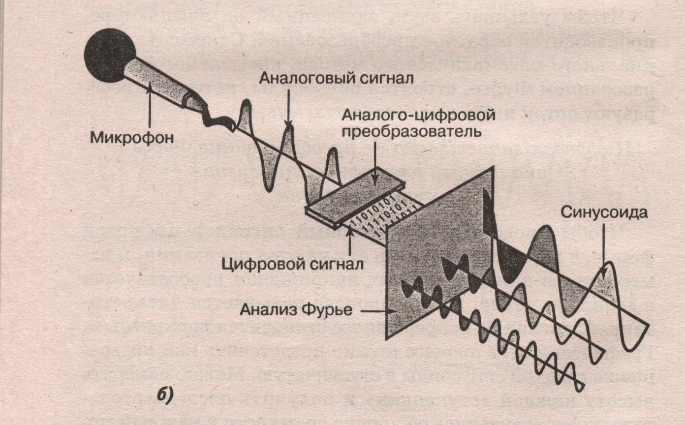
This picture gives the most visual representation of what happens during the Analog Digital Conversion (ADC), and then we will consider why this is necessary, how the technology developed, and what requirements are imposed on such conversion in mobile networks.
Those who have missed or forgotten what was discussed in the first part can recall How we got an electric signal from sound vibrations , and we continue the description of the transformations by moving around the picture, which shows a new area of interest to us at the moment:
First, let's we’ll understand why it is necessary to convert an analog signal into any sequence of zeros and ones that cannot be heard without special knowledge and mathematical transformations.
After the microphone, we have an analog electric signal, which can be easily “voiced” using the speaker, which, in fact, was carried out in the first experiments with telephones: the inverse transformation “electric signal - sound wave” was performed in the same room or at a minimum distance.
Just what is such a phone for? You can bring sound information to the next room without any changes - just raising your voice. Therefore, the task appears - to hear the interlocutor at the maximum distance from the initiator of the conversation.
And here the inexorable laws of nature come into force: the greater the distance, the stronger the electrical signal in the wires damps, and after a certain number of meters / kilometers it will be impossible to restore sound from it.
Those who found city wire phones working with ten-step automatic telephone exchanges (analog telephone exchanges) remember perfectly what voice quality was sometimes provided with the help of these devices. And someone can remember such forgotten exotic inclusions “through a blocker” / “parallel telephone”, when two phones in the same house were connected to one telephone line, while when one subscriber was on the line, the second was forced to wait for the end of his conversation . Believe me - it was not easy!
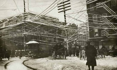
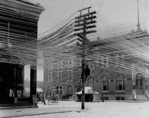
That is, to increase the number of simultaneous calls between two points, using analog lines, we need to lay more and more wires. What this can lead to can be estimated from the urban landscapes of the beginning of the last century:
Therefore, immediately after the invention of the telephone, the best engineers took up the solution of the problem: how to transmit voice over long distances with maximum quality preservation and minimal equipment costs.
What do we need in order for a continuous analog electric signal to turn into a discrete one encoded by sequences of zeros and ones, and at the same time transmit information as close as possible to the original?
A bit of theory.
To convert any analog signal to a digital one, it is necessary to fix the signal amplitude with a certain accuracy (quantization step) at certain intervals (sampling step in the picture below).
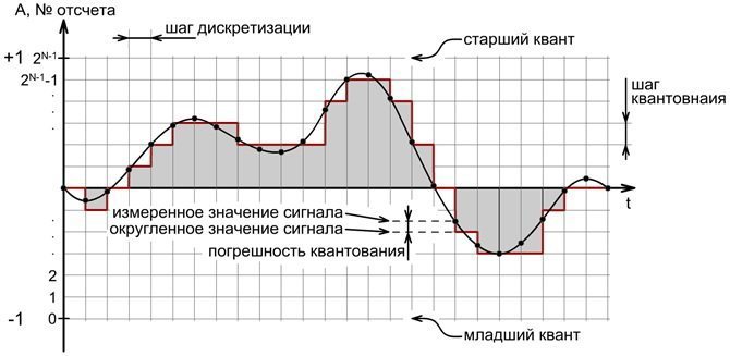
After digitization, we get a stepwise graph, shown in the figure. To maximize the approximation of the digitized signal to the analog, it is necessary to select the sampling step and the quantization step as small as possible, with infinite values we will get a perfectly digitized record.
In practice, infinite digitization accuracy is not required, and you need to choose what accuracy can be considered sufficient to transmit voice with the required quality?
Here, knowledge about the sensitivity of the human organs of hearing will come to our aid: it is generally accepted that a person can distinguish sounds with a frequency from 20 Hz to 22,000 Hz. These are the boundary values for sampling, which will transmit any sound perceived by man. If you translate Hz into more familiar seconds, we get 0.000045 seconds, that is, measurements must be made every 4.5 hundred thousandths of a second! Moreover - and this is not enough. We will talk about the reasons and the required values of the sampling frequency below.
Now we decide on the quantization step: the quantization step allows us to assign at each moment of time a certain amplitude value to the measured signal.
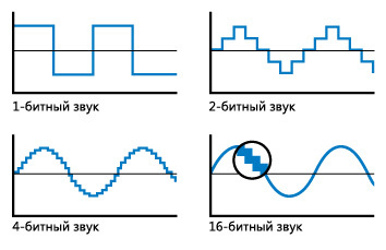
In a first approximation, you can simply check the presence or absence of a signal, to describe such a number of options, we will need only two values: 0 and 1. In computer science, this corresponds to the amount of information: 1 bit and the recording bit rate will be 1. If you digitize any sound with such a bit , at the output we get an intermittent recording, consisting of pauses and the sound of one tone, it can hardly be called a voice recording.
Therefore, it is necessary to increase the number of measured amplitude options, for example, to 4 (that is, to 2 bits - 2 to the power of 2): 0 - 0.25mA - 0.5mA - 0.75mA.
With such values, it will already be possible to distinguish some changes in sound after digitization, and not just its presence or absence. The illustration perfectly illustrates what gives us an increase in bit rate (quantization) when digitizing sound, is shown in this figure:
Now, having seen 44 kHz / 16 bit in the properties of the music file, you can immediately understand that the Analog-Digital Conversion was performed with 1/1 sampling. 44 kHz = 0.000023 seconds and with a quantization depth of 2 to the 16th degree - 65.536 value options.
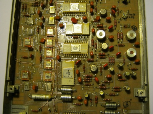
The first circuitry solutions for performing ADC-DAC conversions were, as always, large and slow:
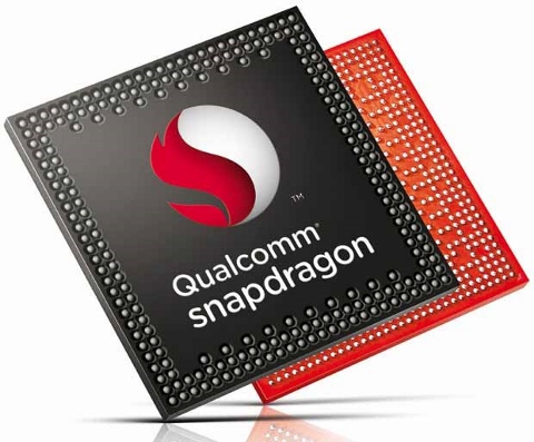
Now these tasks are performed in the main processor of a mobile phone, which simultaneously copes with a huge number of other tasks:
If you digitize without additional optimization of the resulting digital model, the amount of data obtained will be very large, just remember how much space on your disk can take an audio file in an uncompressed form. A standard CD, for example, is 780 megabytes of information and only 74 minutes of sound!
After processing such a file using optimization and compression algorithms with data loss (for example, mp3), the file size can be reduced by 10 or more times.
For our purposes, the amount of data obtained is of fundamental importance, since it still needs to be transmitted to your interlocutor, and the resource of the transport channel is very limited.
Once again, the task for engineers is to maximize the amount of data transferred while maintaining the required quality.
In colloquial speech that sounds during a telephone conversation, the frequency spectrum is much lower than that available for perception, therefore, for transmitting a telephone conversation, you can limit yourself to a narrower spectrum: for example, 50..7000Hz. We wrote about this in sufficient detail in the material on voice codecs in mobile networks.
Now we have the initial data for starting the conversion - an electrical analog signal in the spectrum of 50-7000Hz, and we need to convert the A-CPU, so that the signal distortion during conversion (the very steps on the graph above) does not affect the recording quality . To do this, select the values of the sampling step and quantization step, sufficient for a complete description of the existing analog signal.
Here, one of the fundamental theorems in the field of digital signal processing will come to our aid - Kotelnikov's Theorem .
In it, our compatriot mathematically proved the frequency with which it is necessary to measure the values of a function for its exact numerical representation. For us, the most important consequence of this theorem is the following - measurements need to be carried out twice as often as the highest frequency, which we need to translate into digital form.
Therefore, the sampling step for digitizing a conversation will be enough to take at the level of 14 kHz, and for high-quality digitization of music - 2 x 22 kHz, here we get the standard 44 kHz, with which now, as a rule, music files are created.
There are a wide variety of voice codecs that can be used in wired and wireless networks, and codecs for wired networks generally encode voice with better quality, and codecs for wireless networks (networks of mobile operators) with slightly worse quality.
But these codecs generate additional data to restore the received signal in case of unsuccessful delivery due to complex radio conditions. This feature is called noise immunity, and the development of codecs for mobile networks is in the direction of improving the quality of the transmitted signal while increasing its noise immunity.
In mobile networks, entire classes of voice codecs are used, which include a set of dynamically selected encoding rates, depending on the current position of the subscriber and the quality of the radio coverage at this point:
The table lists all the codecs used in modern mobile networks, of which codecs with a dynamic bitrate (in which the ratio of useful data and redundant data is changed for data recovery) are called AMR - Adaptive Multi Rate. Codecs FR / HR / EFR are used only in GSM networks.
To visualize how much more data is encoded in high-speed codecs, take a look at the following picture:
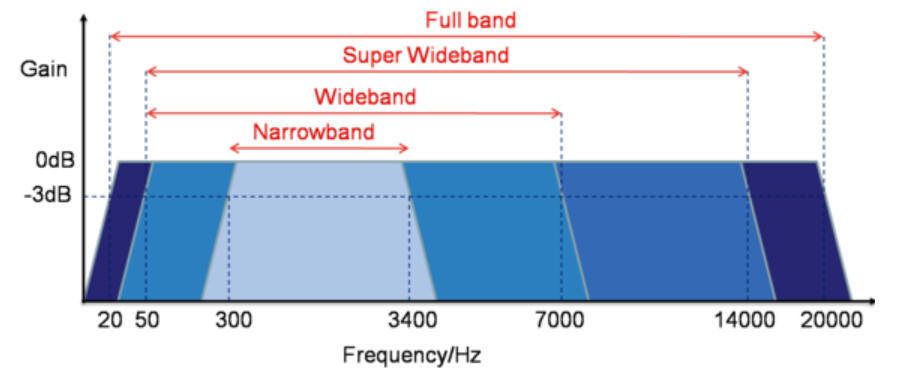
The transition from AMR to AMR-WB codecs almost doubles the amount of data, and AMR-WB + requires another 40-50% more transport channel width!
That is why in mobile networks, broadband codecs in mobile networks have not yet been widely used, but in the future it is possible to switch to the Super Wide Band (AMR-WB +) and even to the Full Band band, for example, for online broadcasts of concerts.
So - after performing the second stage of voice conversion, instead of sound vibrations, we get a stream of digital data, ready for transmission through a transport network.
Until the digit is converted back to an analog signal, this data is stored almost unchanged (sometimes in the process of voice delivery, transcoding from one codec to another can occur), and further conversions that occur with our voice will concern the physical environment through which the call is transmitted.
In the next article, we will consider what happens between the telephone and the base station and how miraculously the data stream we have generated wirelessly is delivered to the operator’s equipment.
PS To everyone who is interested in the topic of digital communication and the history of its development, I highly recommend the book “And the world is mysterious behind the curtain of numbers” by B.I. Kruk, G.N. Popov. From the point of view of modern standards and technologies, it is a little outdated, but the authors describe the theoretical and historical part perfectly, diluting the dry theory with living examples and illustrations.
In order to ensure the transmission of information at any distance without loss of quality, we will need to make a second conversion from an Analog signal to a Digital one.
This picture gives the most visual representation of what happens during the Analog Digital Conversion (ADC), and then we will consider why this is necessary, how the technology developed, and what requirements are imposed on such conversion in mobile networks.
Those who have missed or forgotten what was discussed in the first part can recall How we got an electric signal from sound vibrations , and we continue the description of the transformations by moving around the picture, which shows a new area of interest to us at the moment:
First, let's we’ll understand why it is necessary to convert an analog signal into any sequence of zeros and ones that cannot be heard without special knowledge and mathematical transformations.
After the microphone, we have an analog electric signal, which can be easily “voiced” using the speaker, which, in fact, was carried out in the first experiments with telephones: the inverse transformation “electric signal - sound wave” was performed in the same room or at a minimum distance.
Just what is such a phone for? You can bring sound information to the next room without any changes - just raising your voice. Therefore, the task appears - to hear the interlocutor at the maximum distance from the initiator of the conversation.
And here the inexorable laws of nature come into force: the greater the distance, the stronger the electrical signal in the wires damps, and after a certain number of meters / kilometers it will be impossible to restore sound from it.
Those who found city wire phones working with ten-step automatic telephone exchanges (analog telephone exchanges) remember perfectly what voice quality was sometimes provided with the help of these devices. And someone can remember such forgotten exotic inclusions “through a blocker” / “parallel telephone”, when two phones in the same house were connected to one telephone line, while when one subscriber was on the line, the second was forced to wait for the end of his conversation . Believe me - it was not easy!
That is, to increase the number of simultaneous calls between two points, using analog lines, we need to lay more and more wires. What this can lead to can be estimated from the urban landscapes of the beginning of the last century:
Therefore, immediately after the invention of the telephone, the best engineers took up the solution of the problem: how to transmit voice over long distances with maximum quality preservation and minimal equipment costs.
What do we need in order for a continuous analog electric signal to turn into a discrete one encoded by sequences of zeros and ones, and at the same time transmit information as close as possible to the original?
A bit of theory.
To convert any analog signal to a digital one, it is necessary to fix the signal amplitude with a certain accuracy (quantization step) at certain intervals (sampling step in the picture below).
After digitization, we get a stepwise graph, shown in the figure. To maximize the approximation of the digitized signal to the analog, it is necessary to select the sampling step and the quantization step as small as possible, with infinite values we will get a perfectly digitized record.
In practice, infinite digitization accuracy is not required, and you need to choose what accuracy can be considered sufficient to transmit voice with the required quality?
Here, knowledge about the sensitivity of the human organs of hearing will come to our aid: it is generally accepted that a person can distinguish sounds with a frequency from 20 Hz to 22,000 Hz. These are the boundary values for sampling, which will transmit any sound perceived by man. If you translate Hz into more familiar seconds, we get 0.000045 seconds, that is, measurements must be made every 4.5 hundred thousandths of a second! Moreover - and this is not enough. We will talk about the reasons and the required values of the sampling frequency below.
Now we decide on the quantization step: the quantization step allows us to assign at each moment of time a certain amplitude value to the measured signal.
In a first approximation, you can simply check the presence or absence of a signal, to describe such a number of options, we will need only two values: 0 and 1. In computer science, this corresponds to the amount of information: 1 bit and the recording bit rate will be 1. If you digitize any sound with such a bit , at the output we get an intermittent recording, consisting of pauses and the sound of one tone, it can hardly be called a voice recording.
Therefore, it is necessary to increase the number of measured amplitude options, for example, to 4 (that is, to 2 bits - 2 to the power of 2): 0 - 0.25mA - 0.5mA - 0.75mA.
With such values, it will already be possible to distinguish some changes in sound after digitization, and not just its presence or absence. The illustration perfectly illustrates what gives us an increase in bit rate (quantization) when digitizing sound, is shown in this figure:
Now, having seen 44 kHz / 16 bit in the properties of the music file, you can immediately understand that the Analog-Digital Conversion was performed with 1/1 sampling. 44 kHz = 0.000023 seconds and with a quantization depth of 2 to the 16th degree - 65.536 value options.
The first circuitry solutions for performing ADC-DAC conversions were, as always, large and slow:
Now these tasks are performed in the main processor of a mobile phone, which simultaneously copes with a huge number of other tasks:
If you digitize without additional optimization of the resulting digital model, the amount of data obtained will be very large, just remember how much space on your disk can take an audio file in an uncompressed form. A standard CD, for example, is 780 megabytes of information and only 74 minutes of sound!
After processing such a file using optimization and compression algorithms with data loss (for example, mp3), the file size can be reduced by 10 or more times.
For our purposes, the amount of data obtained is of fundamental importance, since it still needs to be transmitted to your interlocutor, and the resource of the transport channel is very limited.
Once again, the task for engineers is to maximize the amount of data transferred while maintaining the required quality.
In colloquial speech that sounds during a telephone conversation, the frequency spectrum is much lower than that available for perception, therefore, for transmitting a telephone conversation, you can limit yourself to a narrower spectrum: for example, 50..7000Hz. We wrote about this in sufficient detail in the material on voice codecs in mobile networks.
Now we have the initial data for starting the conversion - an electrical analog signal in the spectrum of 50-7000Hz, and we need to convert the A-CPU, so that the signal distortion during conversion (the very steps on the graph above) does not affect the recording quality . To do this, select the values of the sampling step and quantization step, sufficient for a complete description of the existing analog signal.
Here, one of the fundamental theorems in the field of digital signal processing will come to our aid - Kotelnikov's Theorem .
In it, our compatriot mathematically proved the frequency with which it is necessary to measure the values of a function for its exact numerical representation. For us, the most important consequence of this theorem is the following - measurements need to be carried out twice as often as the highest frequency, which we need to translate into digital form.
Therefore, the sampling step for digitizing a conversation will be enough to take at the level of 14 kHz, and for high-quality digitization of music - 2 x 22 kHz, here we get the standard 44 kHz, with which now, as a rule, music files are created.
There are a wide variety of voice codecs that can be used in wired and wireless networks, and codecs for wired networks generally encode voice with better quality, and codecs for wireless networks (networks of mobile operators) with slightly worse quality.
But these codecs generate additional data to restore the received signal in case of unsuccessful delivery due to complex radio conditions. This feature is called noise immunity, and the development of codecs for mobile networks is in the direction of improving the quality of the transmitted signal while increasing its noise immunity.
In mobile networks, entire classes of voice codecs are used, which include a set of dynamically selected encoding rates, depending on the current position of the subscriber and the quality of the radio coverage at this point:
| Codec | Standard | Year of creation | Range of compressible frequencies | Created Bitrate |
|---|---|---|---|---|
| Full Rate - FR | GSM 06.10 | 1990 | 200-3400 Hz | FR 13 kbit / s |
| Half Rate - HR | GSM 06.20 | 1990 | 200-3400 Hz | HR 5.6 kbit / s |
| Enhanced Full Rate - EFR | GSM 06.60 | 1995 | 200-3400 Hz | FR 12.2 kbit / s |
| Adaptive Multi Rate - AMR | 3GPP TS 26.071 | 1999 | 200-3400 Hz | FR 12.20 |
| Adaptive Multi Rate - AMR | 3GPP TS 26.071 | 1999 | 200-3400 Hz | FR 10.20 |
| Adaptive Multi Rate - AMR | 3GPP TS 26.071 | 1999 | 200-3400 Hz | FR / HR 7.95 |
| Adaptive Multi Rate - AMR | 3GPP TS 26.071 | 1999 | 200-3400 Hz | FR / HR 7.40 |
| Adaptive Multi Rate - AMR | 3GPP TS 26.071 | 1999 | 200-3400 Hz | FR / HR 6.70 |
| Adaptive Multi Rate - AMR | 3GPP TS 26.071 | 1999 | 200-3400 Hz | FR / HR 5.90 |
| Adaptive Multi Rate - AMR | 3GPP TS 26.071 | 1999 | 200-3400 Hz | FR / HR 5.15 |
| Adaptive Multi Rate - AMR | 3GPP TS 26.071 | 1999 | 200-3400 Hz | FR / HR 4.75 |
| Adaptive Multi Rate - WideBand, AMR-WB | 3GPP TS 26.190 | 2001 | 50-7000 Hz | FR 23.85 |
| Adaptive Multi Rate - WideBand, AMR-WB | 3GPP TS 26.190 | 2001 | 50-7000 Hz | FR 23.05 |
| Adaptive Multi Rate - WideBand, AMR-WB | 3GPP TS 26.190 | 2001 | 50-7000 Hz | FR 19.85 |
| Adaptive Multi Rate - WideBand, AMR-WB | 3GPP TS 26.190 | 2001 | 50-7000 Hz | FR 18.25 |
| Adaptive Multi Rate - WideBand, AMR-WB | 3GPP TS 26.190 | 2001 | 50-7000 Hz | FR 15.85 |
| Adaptive Multi Rate - WideBand, AMR-WB | 3GPP TS 26.190 | 2001 | 50-7000 Hz | FR 14.25 |
| Adaptive Multi Rate - WideBand, AMR-WB | 3GPP TS 26.190 | 2001 | 50-7000 Hz | FR 12.65 |
| Adaptive Multi Rate - WideBand, AMR-WB | 3GPP TS 26.190 | 2001 | 50-7000 Hz | FR 8.85 |
| Adaptive Multi Rate - WideBand, AMR-WB | 3GPP TS 26.190 | 2001 | 50-7000 Hz | FR 6.60 |
| Adaptive Multi Rate-WideBand +, AMR-WB + | 3GPP TS 26.290 | 2004 | 50-7000 Hz | 6 - 36 kbit / s (mono) |
| Adaptive Multi Rate-WideBand +, AMR-WB + | 3GPP TS 26.290 | 2004 | 50-7000 Hz | 7 - 48 kbit / s (stereo) |
The table lists all the codecs used in modern mobile networks, of which codecs with a dynamic bitrate (in which the ratio of useful data and redundant data is changed for data recovery) are called AMR - Adaptive Multi Rate. Codecs FR / HR / EFR are used only in GSM networks.
To visualize how much more data is encoded in high-speed codecs, take a look at the following picture:
The transition from AMR to AMR-WB codecs almost doubles the amount of data, and AMR-WB + requires another 40-50% more transport channel width!
That is why in mobile networks, broadband codecs in mobile networks have not yet been widely used, but in the future it is possible to switch to the Super Wide Band (AMR-WB +) and even to the Full Band band, for example, for online broadcasts of concerts.
So - after performing the second stage of voice conversion, instead of sound vibrations, we get a stream of digital data, ready for transmission through a transport network.
Until the digit is converted back to an analog signal, this data is stored almost unchanged (sometimes in the process of voice delivery, transcoding from one codec to another can occur), and further conversions that occur with our voice will concern the physical environment through which the call is transmitted.
In the next article, we will consider what happens between the telephone and the base station and how miraculously the data stream we have generated wirelessly is delivered to the operator’s equipment.
PS To everyone who is interested in the topic of digital communication and the history of its development, I highly recommend the book “And the world is mysterious behind the curtain of numbers” by B.I. Kruk, G.N. Popov. From the point of view of modern standards and technologies, it is a little outdated, but the authors describe the theoretical and historical part perfectly, diluting the dry theory with living examples and illustrations.