maisvendoo August 8, 2015 at 16:02

The Magic of Tensor Algebra: Part 18 - Mathematical Modeling of the Janibekov Effect

Content

Introduction

The previous article was supposed to be about the numerical simulation of the Janibekov effect, but it suddenly occurred to me that this effect can be investigated qualitatively, albeit by a fairly approximate first Lyapunov method. However, numerical simulation is also a very interesting question, especially lying in the plane of my research problems. Therefore, today we

Finally, we will determine how to use the Rodrigue-Hamilton parameters to describe the orientation of the body in space
Consider the forms of representation of the equations of motion of a free body: we show how tensor equations can be converted into matrix and component ones.
Let us simulate the motion of a free rigid body with various ratios between the main moments of inertia and show how the Janibekov effect manifests itself.

1. Differential equations of free motion in tensor form

We have repeatedly considered these equations in vector form

$\ begin {align *} & m \, \ vec a_ {c} = \ sum \ vec F_k ^ {\, e} \\ & \ mathbf I_c \, \ vec \ epsilon + \ vec \ omega \ times \ left (\ mathbf I_c \, \ vec \ omega \ right) = \ sum \ vec M_ {c} (\ vec F_k ^ {\, e}) \ end {align *}$

The vector notation is convenient for a general analysis of the nature of dependencies, it is familiar and it shows what a particular term means. However, to further transform the equations into a form convenient for modeling, we turn to tensor notation

$\ begin {align *} & m \, \ left (\ ddot x ^ {\, i} + \ Gamma _ {\, kl} ^ {\, i} \, \ dot x ^ {\, k} \, \ dot x ^ {\, l} \ right) = X ^ {\, i} \\ & I _ {\, j} ^ {\, i} \, \ dot \ omega ^ {j} + \ varepsilon ^ {\, ijk } \, \ omega _ {\, j} \, g _ {\, kl} \, I _ {\, p} ^ {\, l} \, \ omega ^ {\, p} = M ^ {i} \ end {align *}$

where $x ^ {\, i}$ - contravariant coordinates of the center of mass of the body; $X ^ {\, i}$ - contravariant components of the main vector of external forces applied to the body; $M ^ {\, i}$ - contravariant components of the main moment of external forces applied to the body.

The system of equations (2) is already closed, integrating it you can get the law of motion of the center of mass and the dependence of the angular velocity of the body on time. But, we will still be interested in the orientation of the body, so we supplement this system of equations

$2 \, \ varepsilon ^ {\, ijk} \, \ lambda _ {\, j} \, \ dot \ lambda _ {\, k} + 2 \, \ lambda_0 \, \ dot \ lambda ^ {\, i} - 2 \, \ lambda ^ {\, i} \, \ dot \ lambda_0 = \ omega ^ {\, i}$

Equation (3) is nothing more than a representation of the components of the angular velocity through the Rodrigue-Hamilton orientation parameters. We have already received this expression in previous articles . Now we will consider it as a differential equation relating orientation parameters to angular velocity components.

However, the Rodrigue-Hamilton parameters are redundant - there are four of them, and three coordinates are sufficient to describe the orientation of the body in space. And the number of unknowns in system (2), (3) exceeds the number of equations by one. So we will have to supplement equations (2) and (3) with the equation of relationship between the orientation parameters. In the article on the parameters of Rodrigue-Hamilton, we showed that the rotation of the body is conveniently described by a single quaternion, which is

$\ lambda_0 ^ 2 + \ lambda_1 ^ 2 + \ lambda_2 ^ 2 + \ lambda_3 ^ 2 = 1$

or, in tensor form

$\ lambda_0 ^ 2 + \ lambda _ {\, i} \, \ lambda ^ {\, i} = 1$

We differentiate (4) in time

$2 \, \ lambda_0 \, \ dot \ lambda_0 + \ dot \ lambda _ {\, i} \, \ lambda ^ {\, i} + \ lambda _ {\, i} \, \ dot \ lambda ^ {\, i } = 0$

Given the commutativity of the scalar product, we assume $\ dot \ lambda _ {\, i} \, \ lambda ^ {\, i} = \ lambda _ {\, i} \, \ dot \ lambda ^ {\, i}$ then

$\ lambda_0 \, \ dot \ lambda_0 + \ lambda _ {\, i} \, \ dot \ lambda ^ {\, i} = 0$

and there is the desired equation of communication. The complete system of equations of motion of a free rigid body in tensor form will have the form

$\ begin {align *} & \ dot x ^ {\, i} - v ^ {\, i} = 0 \\ & m \, \ left (\ dot v ^ {\, i} + \ Gamma _ {\, kl } ^ {\, i} \, v ^ {\, k} \, v ^ {\, l} \ right) = X ^ {\, i} \\ & 2 \, \ varepsilon ^ {\, ijk} \ , \ lambda _ {\, j} \, \ dot \ lambda _ {\, k} + 2 \, \ lambda_0 \, \ dot \ lambda ^ {\, i} - 2 \, \ lambda ^ {\, i} \ , \ dot \ lambda_0 - \ omega ^ {\, i} = 0 \\ & \ lambda_0 \, \ dot \ lambda_0 + \ lambda _ {\, i} \, \ dot \ lambda ^ {\, i} = 0 \ \ & I _ {\, j} ^ {\, i} \, \ dot \ omega ^ {j} + \ varepsilon ^ {\, ijk} \, \ omega _ {\, j} \, g _ {\, kl} \ , I _ {\, p} ^ {\, l} \, \ omega ^ {\, p} = M ^ {i} \ end {align *}$

Pretty scary - (6) contains 13 first-order nonlinear differential equations with 13 unknown quantities. It looks scary because of the general tensor notation, but when moving to specific coordinates, in our case the Cartesian ones, system (6) will be greatly simplified.

2. The matrix form of the differential equations of motion of a rigid body in a Cartesian basis

We introduce a column vector of the phase coordinates of the body

$\ mathbf y = \ begin {bmatrix} \ mathbf x ^ T && \ mathbf q ^ T && \ mathbf v ^ T && \ mathbf \ omega ^ T \ end {bmatrix} ^ T$

where $\ mathbf x = \ begin {bmatrix} x_c && y_c && z_c \ end {bmatrix} ^ T$ and $\ mathbf v = \ begin {bmatrix} v_ {cx} && v_ {cy} && v_ {cz} \ end {bmatrix} ^ T$ - the position and speed of the center of mass of the body; $\ mathbf q = \ begin {bmatrix} \ lambda_0 && \ lambda_1 && \ lambda_2 && \ lambda_3 \ end {bmatrix} ^ T$ and $\ mathbf \ omega = \ begin {bmatrix} \ omega_x && \ omega_y && \ omega_z \ end {bmatrix} ^ T$ - orientation and angular velocity of the body.

In the Cartesian basis, the metric tensor is represented by the identity matrix and the Christoffel symbols are equal to zero, therefore, system of equations (6) can be written in matrix form as follows

$\ begin {align *} & \ mathbf {\ dot x} - \ mathbf v = \ mathbf 0 \\ & 2 \, \ mathbf B \, \ mathbf {\ dot q} - \ mathbf D \, \ mathbf \ omega = \ mathbf 0 \\ & m \ mathbf {\ dot v} = \ mathbf X \\ & \ mathbf I_c \, \ mathbf {\ dot \ omega} + \ mathbf \ Omega \, \ mathbf I_c \, \ mathbf \ omega = \ mathbf M_c \ end {align *}$

where matrices are introduced

$\ mathbf B = \ begin {bmatrix} \ lambda_0 && \ lambda_1 && \ lambda_2 && \ lambda_3 \\ - \ lambda_1 && \ lambda_0 && - \ lambda_3 && \ lambda_2 \\ - \ lambda_2 && \ lambda_3 & lambda_3 & lambda_3 & lambda_3 & lambda_0 & \\ - \ lambda_3 && - \ lambda_2 && \ lambda_1 && \ lambda_0 \\ \ end {bmatrix}, \ quad \ mathbf D = \ begin {bmatrix} \ mathbf 0 ^ T \\ \ mathbf E \ end {bmatrix}, \ quad \ mathbf \ Omega = \ begin {bmatrix} 0 && - \ omega_z && \ omega_y \\ \ omega_z && 0 && - \ omega_x \\ - \ omega_y && \ omega_z && 0 \ end {bmatrix}$

Solving system (7) with respect to the first derivatives, we obtain

$\ begin {align *} & \ mathbf {\ dot x} = \ mathbf v \\ & \ mathbf {\ dot q} = \ frac {1} {2} \, \ mathbf B ^ {- 1} \, \ mathbf D \, \ mathbf \ omega \\ & \ mathbf {\ dot v} = \ frac {1} {m} \, \ mathbf X \\ & \ mathbf {\ dot \ omega} = \ mathbf I_c ^ {- 1} \, \ left (\ mathbf M_c - \ mathbf \ Omega \, \ mathbf I_c \, \ mathbf \ omega \ right) \ end {align *}$

the system of equations of motion in the form of Cauchy.

3. Modeling the effect of Janibekov

In the absence of external force factors, the right-hand side of system (8) is zero, and the equation of motion of the center of mass is easily integrated, taking into account the initial conditions

$\ mathbf x (t) = \ mathbf x_0 + \ mathbf v_0 \, t$

The rotation of the nut is described by a system of seven first-order equations, which we obtain from (8), introducing dimensionless moments of inertia $i_y = \ frac {I_y} {I_x}$ and $i_z = \ frac {I_z} {I_x}$

$\ begin {align *} & \ dot \ lambda_0 = - \ frac {1} {2} \, \ left (\ lambda_1 \, \ omega_x + \ lambda_2 \, \ omega_y + \ lambda_3 \, \ omega_z \ right) \ \ & \ dot \ lambda_1 = \ frac {1} {2} \, \ left (\ lambda_0 \, \ omega_x + \ lambda_3 \, \ omega_y - \ lambda_2 \, \ omega_z \ right) \\ & \ dot \ lambda_2 = - \ frac {1} {2} \, \ left (\ lambda_3 \, \ omega_x - \ lambda_0 \, \ omega_y - \ lambda_1 \, \ omega_z \ right) \\ & \ dot \ lambda_3 = \ frac {1 } {2} \, \ left (\ lambda_2 \, \ omega_x - \ lambda_1 \, \ omega_y + \ lambda_0 \, \ omega_z \ right) \\ & \ dot \ omega_x = \ left (i_y - i_z) \, \ omega_y \, \ omega_z \\ & \ dot \ omega_y = \ frac {i_z - 1} {i_y} \, \ omega_x \, \ omega_z \\ & \ dot \ omega_z = \ frac {1 - i_y} {i_z} \ , \ omega_x \, \ omega_y \ end {align *}$

For numerical integration of system (9), we set the initial conditions

$\ begin {align *} & \ lambda_0 (0) = 1, \ quad \ lambda_1 (0) = \ lambda_2 (0) = \ lambda_3 (0) = 0 \\ & \ omega_x (0) = \ omega_0, \ quad \ omega_y (0) = \ Delta \ omega_y, \ quad \ omega_z (0) = 0 \ end {align *}$

where $\ omega_0$ is the angular velocity of the nut after leaving the thread; $\ Delta \ omega_y$ - initial angular velocity perturbation

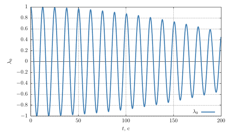
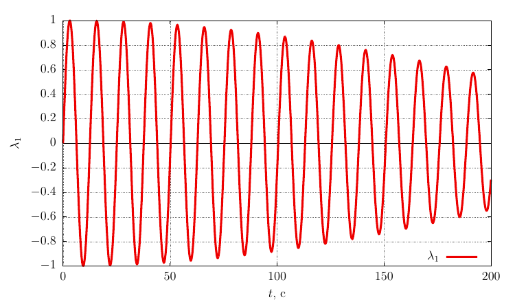
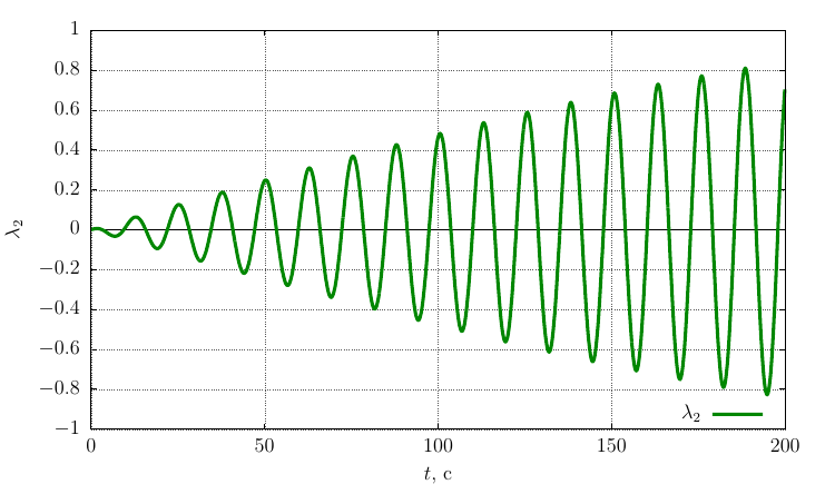
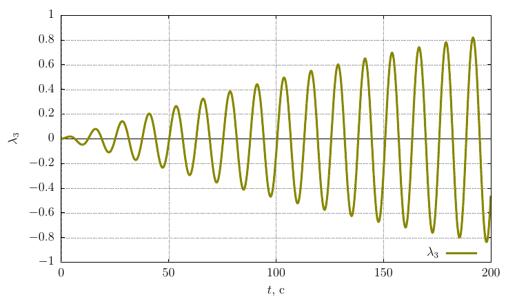
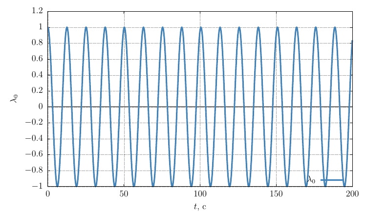
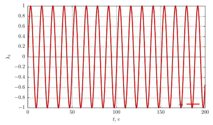
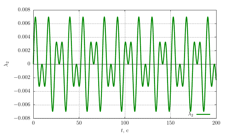
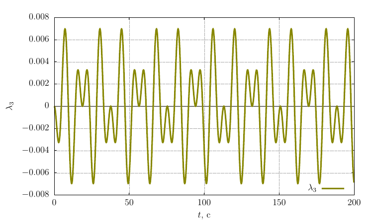
For parameter values $i_y = 2.0, \, i_z = 0.5, \, \ omega_0 = 1.0$ , rad / s, $\ Delta \ omega_y = 1 \ cdot 10 ^ {- 10}$ rad / s, the nut moves as follows:

Rodrigue-Hamilton orientation parameters

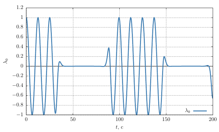
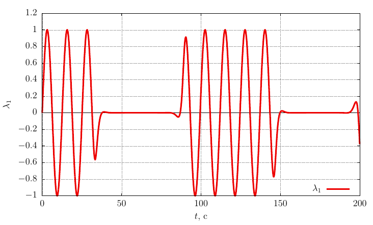
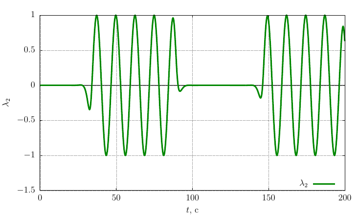
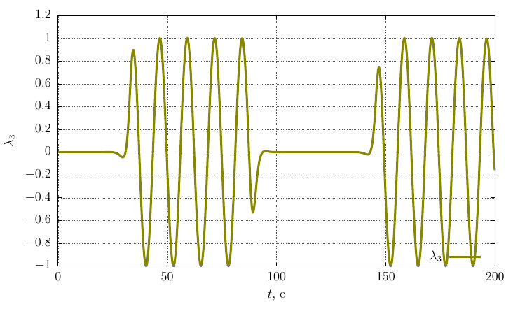
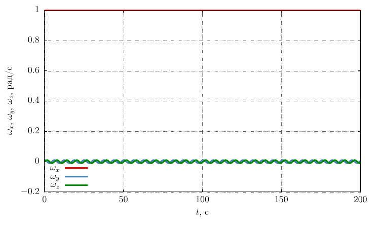
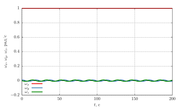
Projections of angular velocity on eigen axes

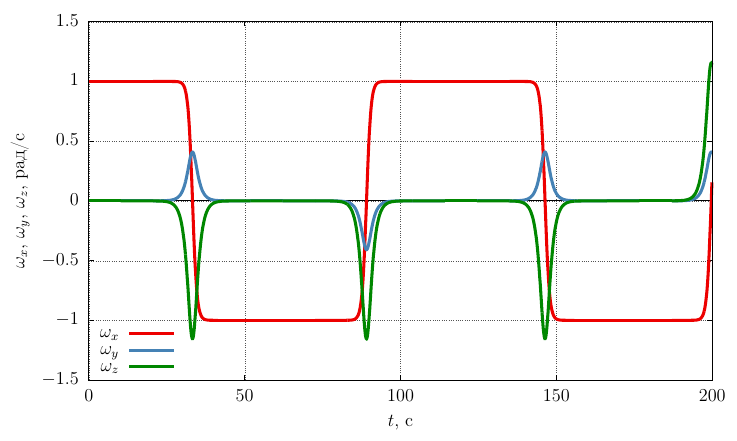
From the graphs it can be seen that, for $I_y> I_x> I_z$ , a very small perturbation of the angular velocity vector leads to periodic an avalanche-like change in the orientation of the nut in space.

Compare the result with the movement of the body twisted around the axis with the maximum moment of inertia, that is, put $I_x> I_y = I_z$ , setting the following parameter values $i_y = 0.5, \, i_z = 0.5, \, \ omega_0 = 1.0$ , rad / s $\ Delta \ omega_y = 1 \ cdot 10 ^ {- 2}$ ,, rad / s

Rodrigue-Hamilton orientation parameters

Projections of the angular velocity on its own axes

It can be seen that, with a sufficiently significant perturbation of the angular velocity, the motion remains stable rotation around the axis $x$ with a small precession.

A similar picture is observed for a body twisted around an axis with a minimum moment of inertia ( $I_x <I_y = I_z$ ) $i_y = 1.5, \, i_z = 1.5, \, \ omega_0 = 1.0$ , rad / s ,, $\ Delta \ omega_y = 1 \ cdot 10 ^ {- 2}$ rad / s

Orientation parameters Rodrigue-Hamilton The

projections of the angular velocity on its own axes

The precession frequency is significantly lower than when twisting around an axis with a maximum moment of inertia, which is logical, since the oscillations occur around the axis with a larger moment of inertia than in the case $I_x> I_y = I_z$ .

Conclusion

All calculations were performed by the author in SKA Maple 18. The graphs are built from the calculation log using the Kile + LaTeX + gnuplot bundle.

I would also like to make an animation, but the author’s experience in this matter is extremely small. Therefore, I would like to ask readers a question - is there software (for Linux / Windows) that can be used to create an animation clip illustrating body movement with a set of values of orientation quaternion parameters depending on time? I suspect that this can be done with Blender 3D, but I'm not sure.

In the meantime, thank you for your attention!

Upd :

Acknowledgments

However, I completely forgot to write that this article (and the previous one) was prepared using the Markdown & LaTeX Editor web application , developed by the user parpalak . This system allows you to type articles in Makdown and LaTeX and generates code suitable for direct insertion into the Habra editor. I am grateful to the author for participating in product testing. With his permission, I recommend this system for use in the preparation of mathematical texts of articles

To be continued ...

Tags: