The formation of musical preferences in the neural network - an experiment to create a smart player
This article is devoted to the study of the ability to train the simplest (relatively) neural network to “listen” to music and to distinguish “good” in the listener's opinion from “bad”.
To teach a neural network to distinguish “bad” music from “good” music or to show that a neural network is incapable of this (this particular implementation of it).

Given that music is a combination of an uncountable number of sounds, it’s impossible to “feed” its neural network just like that, so you need to determine what kind of network will “listen” to it. The options for highlighting the “most important” features from music are endless. It is necessary to determine what needs to be distinguished from the music. As reference data, I determined that you need to highlight some idea of the frequencies of sounds used in music.
I decided to single out the frequencies, because Firstly, they are different for different musical instruments .

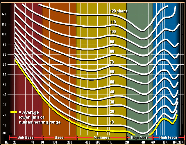
Secondly, the sensitivity of hearing depending on the frequency is different and quite individual (within reasonable limits).
Thirdly, the saturation of the track with certain frequencies is quite individual, but it is similar for similar compositions, for example, guitar solo in two different but similar tracks will give a similar picture of the track “saturation” at the level of individual frequencies.
Thus, the normalization task is reduced to the allocation of some information about the frequencies, which shows:
To select the frequency saturation in the track at each time interval, you can use FFT data, you can manually calculate this data, but I will use the ready-made Bass open library, more precisely, the Bass.NET shell for it , which allows you to get this data more humanely.
To get FFT data from a track, just write a small function .
After receiving the raw data, it is necessary to process them.
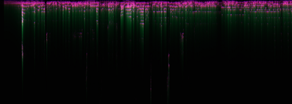
Data visualization
First, you need to determine how many frequency ranges to divide the desired sound, this parameter determines how detailed the analysis result will be, but it will also give a lot of load to the neural network (it will need more neurons to operate with big data). For our task, we take 1024 gradations, this is a rather detailed spectrum of frequencies and a relatively small amount of information at the output. Now it is necessary to determine how to get 1 array from N arrays of float [] that contains more or less all the information we need: the saturation of sound with certain spectra, the frequency of occurrence of various spectra of sound, its volume, its duration.
With the first parameter “saturation”, everything is quite simple, you can simply sum all the arrays and at the output we get how “a lot” there was of each spectrum in the whole track, but this will not reflect other parameters.
In order to “reflect” other parameters as well, it is possible to summarize other parameters a little more complicated, I will not go into details of the implementation of such a “summing” function, because the number of its possible implementations is virtually infinite.
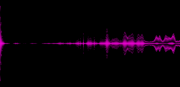
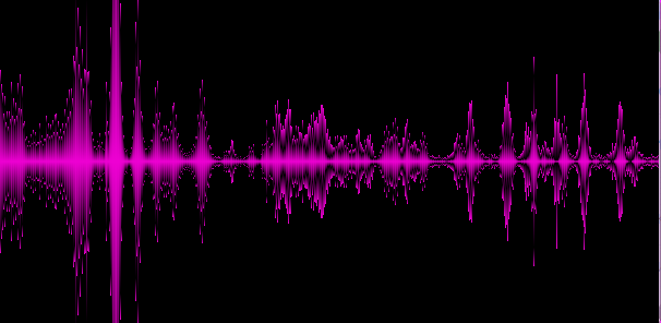
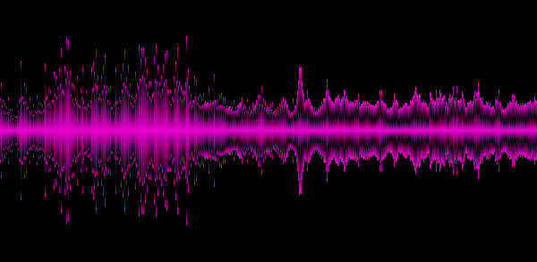
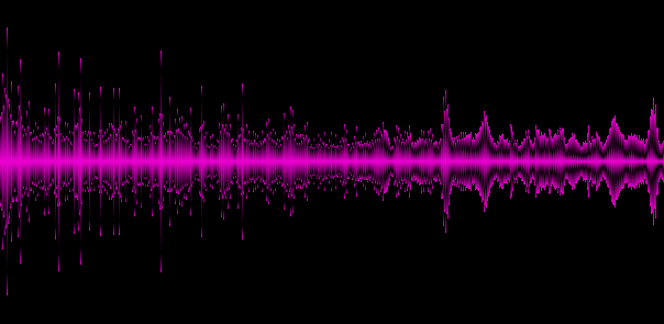
Graphical representation of the resulting array:
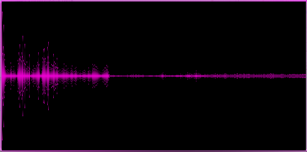
Example 1. Relatively calm melody with elements of light rock, piano and vocals
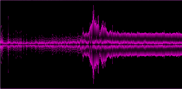
Example 2. Relatively “soft” dubstep with elements ofscrapping the brain from the walls of a not very soft dubstep
Example 3. Music in a style close to trance
Example 4. Pink Floyd
Example 5. Van Halen
Example 6. Anthem of Russia
In the examples given, it becomes clear that different genres give different “spectral patterns”, which is good, so we highlighted at least some key features of the track.
Now we need to prepare the neural network, which we will “train”. There are a lot of neural network algorithms, some are better for certain tasks, some are worse, I do not set a goal to study all types in the context of the task, I will take the first implementation that comes to hand (thanks dr.kernel), flexible enough to adapt to the solution of the task. I don’t choose a “more suitable” neural network, because the task is to check the "neural network" and if its random implementation shows a good result, then there are definitely more suitable types of neural networks, which will show the results even better, if the network fails, it will only show that this neural network failed.
This neural network is trained in data that lies in the range from 0 to 1 and at the output also gives values from 0 to 1. Therefore, the data must be brought to a “suitable form”. You can bring data to a suitable form in many ways, the result will still be similar.
Stage Two: Neural Network Preparation
The neural network that I use is determined by the number of layers, the number of input, output and the number of neurons on each layer.
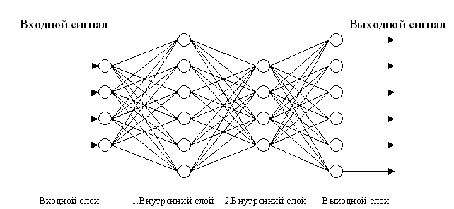
Obviously, not all configurations are “equally useful”, but I don’t know of any methods, if any, for determining the “best” configuration for this task. One could just try a few different configurations and focus on the one that “suits better”, but I will go the other way, I will grow a neural network with an evolutionary algorithm, later in the article I will explain how.
At this point, the format of the input data is defined, you need to determine the format of the output data. Obviously, you can simply divide the tracks into “good” and “bad” and 1 output neuron will be enough, but I think that the good and bad concept is extensible, in particular, certain music is better for waking up in the morning, another walk around the city on the way to work, the third for rest in the evening after work, etc. that is, the quality of the track should also be determined relative to the time of day and day of the week, total 24 * 7 output neurons.
Now you need to determine the sample for training, for this you can of course take all the tracks and sit and note at what time you want to listen to them or better never to hear, but I'm not one of those who would sit for hours and mark the tracks, it’s much easier to do it “along the way” plays ”, that is, while listening to the track. That is, the “training” sample should be formed by the player, while listening to the tracks in which the track could be marked as “good” or “bad”. And so imagine that there is such a player (it really is, that is, it was written based on the open source codes of another player). After ten hours of listening to music on various days, data is collected for the first sample. Each sample element contains input data (1024 values of the spectral picture of the track) and output (24 * 7 values from 0 to 1, where 0 is a really bad track and 1 is a very good track for every hour of 7 days of the week). At the same time, at “good” track + was set on all days of the week and hours, but at this hour \ day of the week + was larger, and similarly for “bad”, that is, the data is not 0 and 1, but some values are between 0 and 1 .
There is data for training, now we need to determine what to consider a trained network, in this case we can assume that for the data loaded into it, the difference between the network response to the input data should not be minimal and the initial output data. The ability of the network to “predict” from data unknown to it is also extremely important, that is, it should not be retrained, there will be little sense in retraining the network. There are no problems to determine the “response quality”, for this there is a function calculating the error, the question remains how to determine the quality of the prediction. To solve this problem, it is enough to train the network on 1 sample, but check the quality on another, while the samples should be random and the elements of the first and second should not be repeated.
An algorithm for checking the level of network learning is found, now you need to determine its configuration. As I said, an evolutionary algorithm will be used for this. To do this, take the starting configuration, say 10 layers, each with 100 neurons (this will definitely be small and the quality of such a network will not be very good), then we will train for a certain number of steps (say 1000), after we determine the quality of its training. Next, we move on to “evolution”, create 10 configurations, each of which is a “mutant” of the original, that is, it has a randomly changed either the number of layers or the number of neurons on each or some layers. Next, we train each configuration in the same way as the original one, select the best one and define it as the original one. We continue this process until such a moment comes, that we cannot find a configuration that learns better than the original. We consider this configuration the best, it turned out to be the best able to “remember” the initial data and predicts best of all, that is, the result of its training is the highest quality possible.
The evolutionary process took about 6 hours for a sample of 6000 elements in size, after a couple of hours of optimizations, the process takes about 30 minutes, the configuration may differ in different samples, but most often the configuration is about 7 layers, with the number of neurons gradually increasing to 3-4 layers and further, it shrinks more quickly to the last layer, a kind of hump on 3-4 layers out of 7, apparently this configuration is the most “capable” for a given network.
So the network has “grown” and is capable of learning, the usual learning for the network begins, long and tedious (up to 15 minutes), after which the network is ready to “listen to music” and say “bad” or “good”.
The weight of the “brain” - configuration of the trained network was 25 mb, the weight will vary for different samples, in general, the larger the sample, the more neurons are needed to deal with it, but the weight of the average network will be about the same.

The training sample consisted of “good” tracks in my humble opinion, such as Van Halen, Pink Floyd, classical music (not any), soft rock, melodic and calm tracks. In my opinion, “bad” in the sample was considered rap, pop, too hard rock.
We define the “quality index” of random tracks, which the neural network will calculate after training.
The first neural network, after the “evolutionary” configuration and training settings showed the presence of “skills” to determine the characteristics of the track. A neural network can be taught to “listen to music” and separate tracks that the “listener” who taught it will like or dislike.
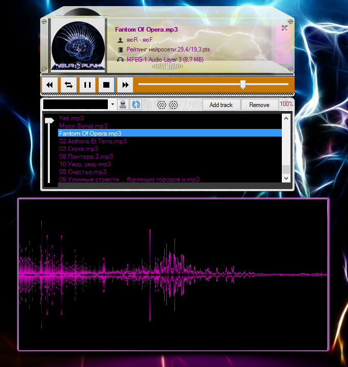
The full source code of the application in C # and the compiled version can be downloaded on GitHub or via Sync .
Appearance of the application , which implements all the functionality described in the article:
I hope that my experience in this study will help in the future for those who want to explore the capabilities of neural networks.
goal
To teach a neural network to distinguish “bad” music from “good” music or to show that a neural network is incapable of this (this particular implementation of it).
Stage One: Data Normalization
Given that music is a combination of an uncountable number of sounds, it’s impossible to “feed” its neural network just like that, so you need to determine what kind of network will “listen” to it. The options for highlighting the “most important” features from music are endless. It is necessary to determine what needs to be distinguished from the music. As reference data, I determined that you need to highlight some idea of the frequencies of sounds used in music.
I decided to single out the frequencies, because Firstly, they are different for different musical instruments .
Secondly, the sensitivity of hearing depending on the frequency is different and quite individual (within reasonable limits).
Thirdly, the saturation of the track with certain frequencies is quite individual, but it is similar for similar compositions, for example, guitar solo in two different but similar tracks will give a similar picture of the track “saturation” at the level of individual frequencies.
Thus, the normalization task is reduced to the allocation of some information about the frequencies, which shows:
- how often does sound from a given frequency range sound in a composition
- how loud he sounded
- how long did he sound
- and so for each specific frequency range (you need to break the entire "audible" spectrum into a certain number of ranges).
To select the frequency saturation in the track at each time interval, you can use FFT data, you can manually calculate this data, but I will use the ready-made Bass open library, more precisely, the Bass.NET shell for it , which allows you to get this data more humanely.
To get FFT data from a track, just write a small function .
After receiving the raw data, it is necessary to process them.
Data visualization
First, you need to determine how many frequency ranges to divide the desired sound, this parameter determines how detailed the analysis result will be, but it will also give a lot of load to the neural network (it will need more neurons to operate with big data). For our task, we take 1024 gradations, this is a rather detailed spectrum of frequencies and a relatively small amount of information at the output. Now it is necessary to determine how to get 1 array from N arrays of float [] that contains more or less all the information we need: the saturation of sound with certain spectra, the frequency of occurrence of various spectra of sound, its volume, its duration.
With the first parameter “saturation”, everything is quite simple, you can simply sum all the arrays and at the output we get how “a lot” there was of each spectrum in the whole track, but this will not reflect other parameters.
In order to “reflect” other parameters as well, it is possible to summarize other parameters a little more complicated, I will not go into details of the implementation of such a “summing” function, because the number of its possible implementations is virtually infinite.
Graphical representation of the resulting array:
Example 1. Relatively calm melody with elements of light rock, piano and vocals
Example 2. Relatively “soft” dubstep with elements of
Example 3. Music in a style close to trance
Example 4. Pink Floyd
Example 5. Van Halen
Example 6. Anthem of Russia
In the examples given, it becomes clear that different genres give different “spectral patterns”, which is good, so we highlighted at least some key features of the track.
Now we need to prepare the neural network, which we will “train”. There are a lot of neural network algorithms, some are better for certain tasks, some are worse, I do not set a goal to study all types in the context of the task, I will take the first implementation that comes to hand (thanks dr.kernel), flexible enough to adapt to the solution of the task. I don’t choose a “more suitable” neural network, because the task is to check the "neural network" and if its random implementation shows a good result, then there are definitely more suitable types of neural networks, which will show the results even better, if the network fails, it will only show that this neural network failed.
This neural network is trained in data that lies in the range from 0 to 1 and at the output also gives values from 0 to 1. Therefore, the data must be brought to a “suitable form”. You can bring data to a suitable form in many ways, the result will still be similar.
Stage Two: Neural Network Preparation
The neural network that I use is determined by the number of layers, the number of input, output and the number of neurons on each layer.
Obviously, not all configurations are “equally useful”, but I don’t know of any methods, if any, for determining the “best” configuration for this task. One could just try a few different configurations and focus on the one that “suits better”, but I will go the other way, I will grow a neural network with an evolutionary algorithm, later in the article I will explain how.
At this point, the format of the input data is defined, you need to determine the format of the output data. Obviously, you can simply divide the tracks into “good” and “bad” and 1 output neuron will be enough, but I think that the good and bad concept is extensible, in particular, certain music is better for waking up in the morning, another walk around the city on the way to work, the third for rest in the evening after work, etc. that is, the quality of the track should also be determined relative to the time of day and day of the week, total 24 * 7 output neurons.
Now you need to determine the sample for training, for this you can of course take all the tracks and sit and note at what time you want to listen to them or better never to hear, but I'm not one of those who would sit for hours and mark the tracks, it’s much easier to do it “along the way” plays ”, that is, while listening to the track. That is, the “training” sample should be formed by the player, while listening to the tracks in which the track could be marked as “good” or “bad”. And so imagine that there is such a player (it really is, that is, it was written based on the open source codes of another player). After ten hours of listening to music on various days, data is collected for the first sample. Each sample element contains input data (1024 values of the spectral picture of the track) and output (24 * 7 values from 0 to 1, where 0 is a really bad track and 1 is a very good track for every hour of 7 days of the week). At the same time, at “good” track + was set on all days of the week and hours, but at this hour \ day of the week + was larger, and similarly for “bad”, that is, the data is not 0 and 1, but some values are between 0 and 1 .
There is data for training, now we need to determine what to consider a trained network, in this case we can assume that for the data loaded into it, the difference between the network response to the input data should not be minimal and the initial output data. The ability of the network to “predict” from data unknown to it is also extremely important, that is, it should not be retrained, there will be little sense in retraining the network. There are no problems to determine the “response quality”, for this there is a function calculating the error, the question remains how to determine the quality of the prediction. To solve this problem, it is enough to train the network on 1 sample, but check the quality on another, while the samples should be random and the elements of the first and second should not be repeated.
An algorithm for checking the level of network learning is found, now you need to determine its configuration. As I said, an evolutionary algorithm will be used for this. To do this, take the starting configuration, say 10 layers, each with 100 neurons (this will definitely be small and the quality of such a network will not be very good), then we will train for a certain number of steps (say 1000), after we determine the quality of its training. Next, we move on to “evolution”, create 10 configurations, each of which is a “mutant” of the original, that is, it has a randomly changed either the number of layers or the number of neurons on each or some layers. Next, we train each configuration in the same way as the original one, select the best one and define it as the original one. We continue this process until such a moment comes, that we cannot find a configuration that learns better than the original. We consider this configuration the best, it turned out to be the best able to “remember” the initial data and predicts best of all, that is, the result of its training is the highest quality possible.
The evolutionary process took about 6 hours for a sample of 6000 elements in size, after a couple of hours of optimizations, the process takes about 30 minutes, the configuration may differ in different samples, but most often the configuration is about 7 layers, with the number of neurons gradually increasing to 3-4 layers and further, it shrinks more quickly to the last layer, a kind of hump on 3-4 layers out of 7, apparently this configuration is the most “capable” for a given network.
So the network has “grown” and is capable of learning, the usual learning for the network begins, long and tedious (up to 15 minutes), after which the network is ready to “listen to music” and say “bad” or “good”.
Stage Three: Collecting Results
The weight of the “brain” - configuration of the trained network was 25 mb, the weight will vary for different samples, in general, the larger the sample, the more neurons are needed to deal with it, but the weight of the average network will be about the same.
The training sample consisted of “good” tracks in my humble opinion, such as Van Halen, Pink Floyd, classical music (not any), soft rock, melodic and calm tracks. In my opinion, “bad” in the sample was considered rap, pop, too hard rock.
We define the “quality index” of random tracks, which the neural network will calculate after training.
- Van Halen - 29 pts
- Rammstein-Mutter (album) - 20-23 pts
- Rihanna - 26 pts
- The Punisher -11-17 pts
- Radiorama - 25 pts
- R Claudermann - 25-29 pts
- The Gregorians - 27-29 pts
- Pink Floyd - 29-33 pts
- Russian rap of low quality - 9-11 pts
- Red mold 16-19 pts
- Bi-2 24-29 pts
- Leap Year - 25-33 pts
Conclusion:
The first neural network, after the “evolutionary” configuration and training settings showed the presence of “skills” to determine the characteristics of the track. A neural network can be taught to “listen to music” and separate tracks that the “listener” who taught it will like or dislike.
The full source code of the application in C # and the compiled version can be downloaded on GitHub or via Sync .
Appearance of the application , which implements all the functionality described in the article:
I hope that my experience in this study will help in the future for those who want to explore the capabilities of neural networks.