Dynamic programming or "Divide and Conquer"
This article discusses the similarities and differences between the two approaches to solving algorithmic problems: dynamic programming (dynamic programming) and the principle of "divide and conquer" (divide and conquer). Comparison will be done using the example of two algorithms, respectively: binary search (how to quickly find a number in a sorted array) and Levenshtein distance (how to convert one line to another with the minimum number of operations).
I want to immediately note that this comparison and explanation does not claim exceptional accuracy. And maybe even some university professors would like to deduct me :) This article is just my personal attempt to sort things out and understand what dynamic programming is and how the principle of “divide and conquer” participates.
So let's get started ...

When I began to study algorithms, it was difficult for me to understand the basic idea of dynamic programming (hereinafter referred to as DP , from Dynamic Programming) and how it differs from the divide and conquer approach (hereinafter DC , from divide-and-conquer). When it comes to comparing these two paradigms, many usually successfully use the Fibonacci function to illustrate. And this is a great illustration. But it seems to me that when we use the same task to illustrate DP and DC, we lose one important detail that can help us catch the difference between the two approaches faster. And this detail consists in the fact that these two techniques are best manifested in solving various types of problems.
I am still in the process of studying DP and DC and cannot say that I fully understood these concepts. But I still hope that this article will shed additional light and help to make another step in the study of such significant approaches as dynamic programming and divide-and-conquer.
The way I see these two concepts now, I can conclude that DP is an extended version of DC .
I would not consider them something completely different. Because both of these concepts recursively divide the problem into two or more subproblems of the same type , until these subproblems are light enough to solve them head-on, directly. Further, all solutions to subproblems are combined together in order to ultimately give an answer to the original, original problem.
So why then do we still have two different approaches (DP and DC) and why I called dynamic programming an extension. This is because dynamic programming can be applied to tasks that have certaincharacteristics and limitations . And only in this case, DP expands DC with two techniques: memoization and tabulation .
Let's get into the details a bit ...
As we have just figured out with you, there are two key characteristics that a task / problem must have in order for us to try to solve it using dynamic programming:
As soon as we can find these two characteristics in the problem we are considering, we can say that it can be solved using dynamic programming.
DP extends DC with the help of two techniques ( memoization and tabulation ), the purpose of which is to preserve sub-solutions to their further reuse. Thus, solutions to subproblems are cached, which leads to a significant improvement in the performance of the algorithm. For example, the time complexity of the “naive” recursive implementation of the Fibonacci function - . At the same time, a solution based on dynamic programming is executed only in time . Memoization (top-down cache filling) is a caching technique that re-uses previously calculated subtask solutions. The Fibonacci function using the memoization technique would look like this:
Tabulation (filling the cache from bottom to top) is a similar technique, but which is primarily focused on filling the cache, and not on finding a solution to sub-problems. Calculation of values that need to be placed in the cache is easiest in this case to perform iteratively, and not recursively. The Fibonacci function using the tabbing technique would look like this:
You can read more about comparison of memoization and tabulation here .
The basic idea that needs to be grasped in these examples is that since our DC problem has overlapping subproblems, we can use solution caching of subproblems using one of two caching techniques: memoization and tabulation.
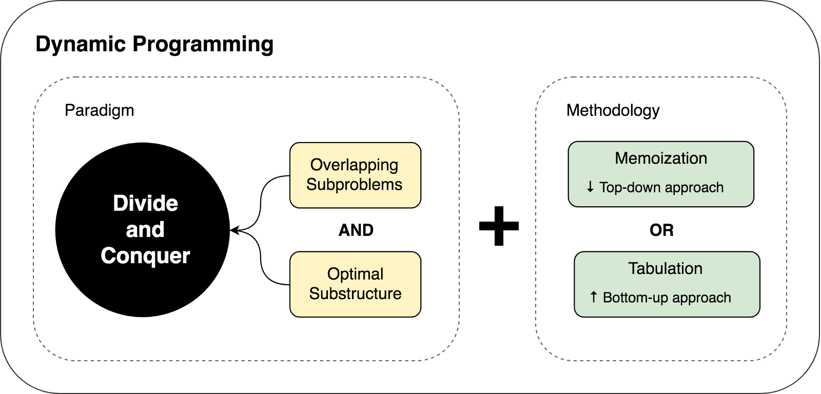
We familiarized with the limitations and prerequisites of using dynamic programming, as well as with the caching techniques used in the DP approach. Let's try to summarize and portray the above thoughts in the following illustration:
Let's try to solve a couple of problems using DP and DC to demonstrate both of these approaches in action.
The binary search algorithm is a search algorithm that finds the position of the requested item in a sorted array. In binary search, we compare the value of the desired variable with the value of the element in the middle of the array. If they are not equal, then half of the array in which the search element cannot be excluded from further search. The search continues in that half of the array, in which the desired variable can be found until it is found. If the next half of the array does not contain elements, the search is considered complete and we conclude that the array does not contain the desired value.
Example
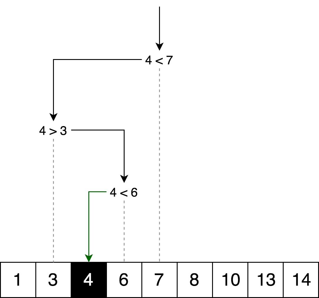
The illustration below is an example of a binary search for the number 4 in an array.
Let's draw the same search logic, but in the form of a decision tree.
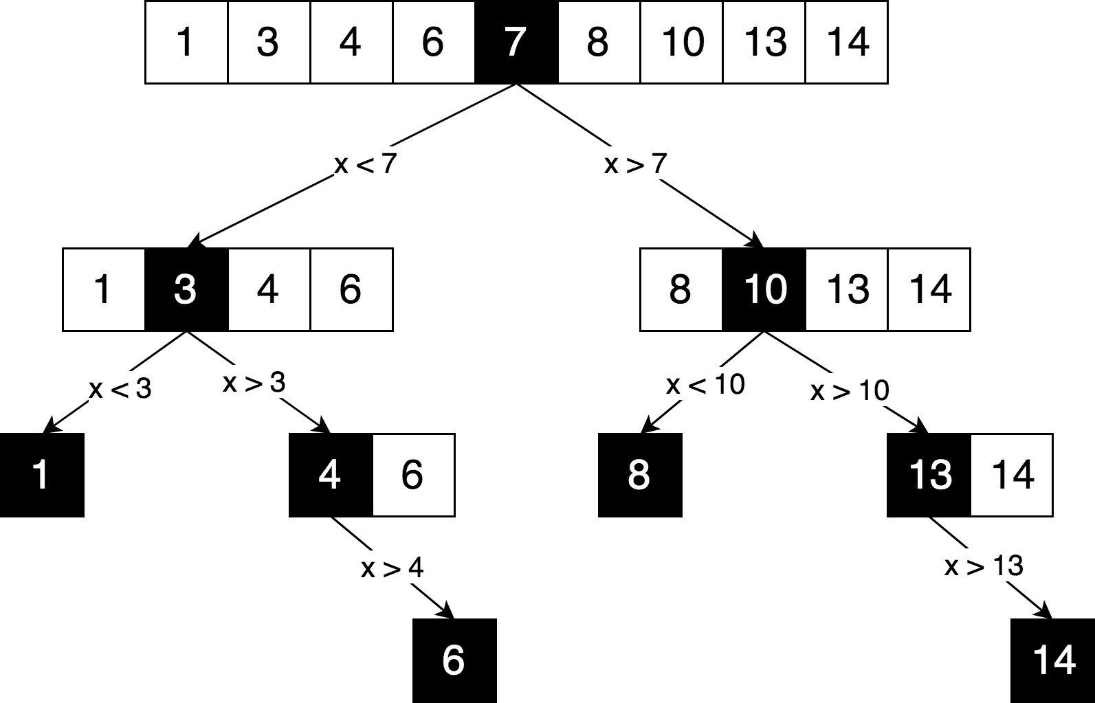
You can see in this scheme a clear “divide and conquer” principle used to solve this problem. We iteratively break our original array into sub-arrays and try to find the desired element already in them.
Can we solve this problem using dynamic programming? No . For the reason that this task does not contain overlapping subproblems . Each time we break an array into parts, both parts are completely independent and not intersecting. And according to the assumptions and limitations of dynamic programming that we discussed above, the subproblems must somehow intersect, they must be repetitive .
Usually, whenever a decision tree looks exactly liketree (and not as a graph ), it most likely means the absence of overlapping subproblems.
Implementation of the algorithm.
Here you can find the full source code of the binary search algorithm with tests and explanations.
Usually, when it comes to explaining dynamic programming, the Fibonacci function is used as an example . But in our case, let's take a slightly more complex example. The more examples, the easier it is to understand the concept.
The editing distance (or Levenshtein distance) between two lines is the minimum number of operations to insert one character, delete one character, and replace one character with another, necessary to turn one line into another.
Example
For example, the editing distance between the words “kitten” and “sitting” is 3, since it is necessary to perform three editing operations (two replacements and one insert) in order to convert one line to another. And it is impossible to find a faster conversion option with fewer operations:
Application of the algorithm
The algorithm has a wide range of applications, for example, for spell checking, systems for correcting optical recognition, inaccurate string search, etc. The
mathematical definition of a problem
Mathematically Levenshtein distance between two lines

Pay attention , the first line in the function
Explanation
Let's try to figure out what this formula tells us. Take a simple example of finding the minimum editing distance between ME and MY lines . Intuitively, you already know that the minimum editing distance equals one ( 1 ) replacement operation (replace “E” with “Y”). But let's formalize our solution and turn it into an algorithmic form in order to be able to solve more complex versions of this problem, such as transforming the word Saturday into Sunday .
In order to apply the formula to the transformation ME → MY, we first need to know the minimum editing distance between ME → M, M → MY and M → M. Next, we must choose the minimum distance from three distances and add one operation (+1) to the transformation E → Y to it.
So, we can already see the recursive nature of this solution: the minimum editing distance ME → MY is calculated based on the three previous possible transformations. Thus, we can already say that this is a divide-and-conquer algorithm.
To further explain the algorithm, let's put two of our rows in the matrix:
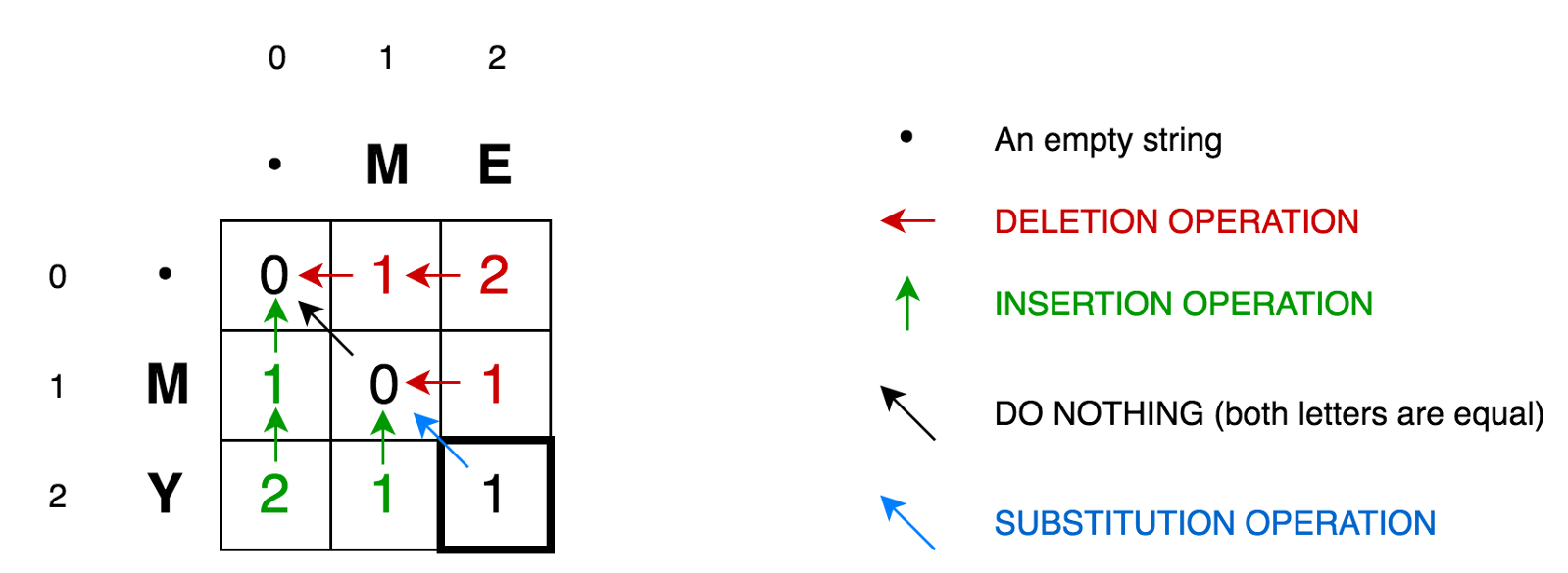
Cell (0,1) contains the red number 1. This means, we need to perform 1 operation in order to convert M to the empty string - remove M. Therefore, we denoted this number in red.
Cell (0,2) contains the red number 2. This means that we need to perform 2 operations in order to transform the string ME into an empty line — delete E, delete M.
Cell (1.0) contains the green number 1. This means that we need 1 operation to transform the empty string into M - insert M. We marked the insert operation in green.
The cell (2,0) contains the green number 2. This means that we need to perform 2 operations in order to convert the empty string to the string MY - insert Y, insert M.
Cell (1.1) contains the number 0. This means that we do not need to do any operation in order to convert the string M to M.
Cell (1,2)contains the red number 1. This means that we need to perform 1 operation in order to transform the ME line into M - delete E.
And so on ...
It does not look difficult for small matrices like ours (only 3x3). But how can we calculate the values of all the cells for large matrices (such as for a 9x7 matrix with the transformation Saturday → Sunday)?
The good news is that, according to the formula, all that we need to calculate the value of any cell with the coordinates
So again, you can clearly see the recursive nature of this task.

We also saw that we were dealing with a divide-and-conquer task. But, can we apply dynamic programming to solve this problem? Does this task satisfy the above-mentioned conditions of “ overlapping problems ” and “ optimal substructures ”? Yes . Let's build a decision tree.

First, you may notice that our decision tree looks more like a decision graph , rather than a tree . You may also notice several intersecting subtasks.. It is also clear that it is impossible to reduce the number of operations and make it smaller than the number of operations from those three neighboring cells (subproblems).
You may also notice that the value in each cell is calculated based on the previous values. Thus, in this case, the tabulation technique is used (filling the cache in the bottom-up direction). You will see this in the sample code below.
Applying all these principles, we can solve more complex problems, for example the transformation task Saturday → Sunday: Here is a
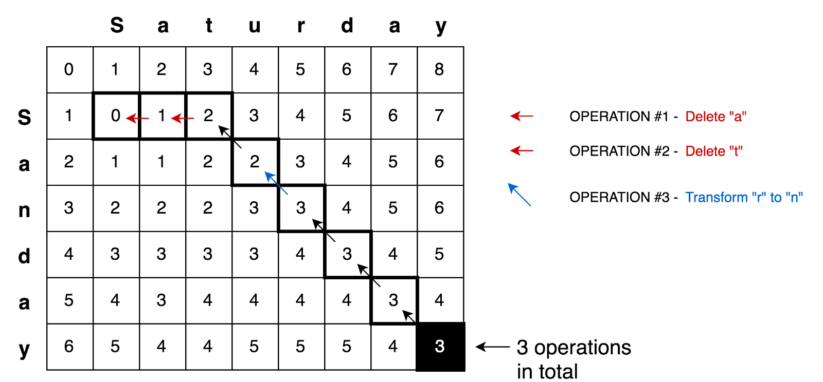
sample of the code
where you can find a complete solution for finding the minimum editing distance with tests and explanations:
In this article, we compared two algorithmic approaches (“dynamic programming” and “divide and conquer”) to solving problems. We found that dynamic programming uses the “divide and conquer” principle and can be applied to problem solving if the task contains intersecting subproblems and an optimal substructure (as is the case with Levenshtein distance). Dynamic programming further uses memoization and tabulation techniques to save submissions for further reuse.
I hope this article clarified rather than complicated the situation for those of you who tried to deal with such important concepts as dynamic programming and “divide and rule” :)
You can find more algorithmic examples using dynamic programming with tests and explanations in the JavaScript Algorithms and Data Structures repository .
Successful coding!
I want to immediately note that this comparison and explanation does not claim exceptional accuracy. And maybe even some university professors would like to deduct me :) This article is just my personal attempt to sort things out and understand what dynamic programming is and how the principle of “divide and conquer” participates.
So let's get started ...

Problem
When I began to study algorithms, it was difficult for me to understand the basic idea of dynamic programming (hereinafter referred to as DP , from Dynamic Programming) and how it differs from the divide and conquer approach (hereinafter DC , from divide-and-conquer). When it comes to comparing these two paradigms, many usually successfully use the Fibonacci function to illustrate. And this is a great illustration. But it seems to me that when we use the same task to illustrate DP and DC, we lose one important detail that can help us catch the difference between the two approaches faster. And this detail consists in the fact that these two techniques are best manifested in solving various types of problems.
I am still in the process of studying DP and DC and cannot say that I fully understood these concepts. But I still hope that this article will shed additional light and help to make another step in the study of such significant approaches as dynamic programming and divide-and-conquer.
DP and DC similarity
The way I see these two concepts now, I can conclude that DP is an extended version of DC .
I would not consider them something completely different. Because both of these concepts recursively divide the problem into two or more subproblems of the same type , until these subproblems are light enough to solve them head-on, directly. Further, all solutions to subproblems are combined together in order to ultimately give an answer to the original, original problem.
So why then do we still have two different approaches (DP and DC) and why I called dynamic programming an extension. This is because dynamic programming can be applied to tasks that have certaincharacteristics and limitations . And only in this case, DP expands DC with two techniques: memoization and tabulation .
Let's get into the details a bit ...
Limitations and characteristics required for dynamic programming
As we have just figured out with you, there are two key characteristics that a task / problem must have in order for us to try to solve it using dynamic programming:
- Optimal substructure - it should be possible to make the optimal solution of the problem from the optimal solution of its subtasks.
- Intersecting subproblems - the problem must be broken down into subproblems, which in turn are reused many times. In other words, a recursive approach to solving a problem would suggest a multiple ( non -one-time) solution of the same sub-problem, instead of producing new and unique sub-problems in each recursive cycle.
As soon as we can find these two characteristics in the problem we are considering, we can say that it can be solved using dynamic programming.
Dynamic programming as an extension of the divide and conquer principle
DP extends DC with the help of two techniques ( memoization and tabulation ), the purpose of which is to preserve sub-solutions to their further reuse. Thus, solutions to subproblems are cached, which leads to a significant improvement in the performance of the algorithm. For example, the time complexity of the “naive” recursive implementation of the Fibonacci function - . At the same time, a solution based on dynamic programming is executed only in time . Memoization (top-down cache filling) is a caching technique that re-uses previously calculated subtask solutions. The Fibonacci function using the memoization technique would look like this:
O(2n)О(n)memFib(n) {
if (mem[n] is undefined)
if (n < 2) result = n
else result = memFib(n-2) + memFib(n-1)
mem[n] = result
return mem[n]
}Tabulation (filling the cache from bottom to top) is a similar technique, but which is primarily focused on filling the cache, and not on finding a solution to sub-problems. Calculation of values that need to be placed in the cache is easiest in this case to perform iteratively, and not recursively. The Fibonacci function using the tabbing technique would look like this:
tabFib(n) {
    mem[0] = 0
    mem[1] = 1for i = 2...n
        mem[i] = mem[i-2] + mem[i-1]
    return mem[n]
}
You can read more about comparison of memoization and tabulation here .
The basic idea that needs to be grasped in these examples is that since our DC problem has overlapping subproblems, we can use solution caching of subproblems using one of two caching techniques: memoization and tabulation.
So what is the difference between DP and DC in the end?
We familiarized with the limitations and prerequisites of using dynamic programming, as well as with the caching techniques used in the DP approach. Let's try to summarize and portray the above thoughts in the following illustration:

Let's try to solve a couple of problems using DP and DC to demonstrate both of these approaches in action.
An example of the principle of "divide and conquer": Binary search
The binary search algorithm is a search algorithm that finds the position of the requested item in a sorted array. In binary search, we compare the value of the desired variable with the value of the element in the middle of the array. If they are not equal, then half of the array in which the search element cannot be excluded from further search. The search continues in that half of the array, in which the desired variable can be found until it is found. If the next half of the array does not contain elements, the search is considered complete and we conclude that the array does not contain the desired value.
Example
The illustration below is an example of a binary search for the number 4 in an array.

Let's draw the same search logic, but in the form of a decision tree.

You can see in this scheme a clear “divide and conquer” principle used to solve this problem. We iteratively break our original array into sub-arrays and try to find the desired element already in them.
Can we solve this problem using dynamic programming? No . For the reason that this task does not contain overlapping subproblems . Each time we break an array into parts, both parts are completely independent and not intersecting. And according to the assumptions and limitations of dynamic programming that we discussed above, the subproblems must somehow intersect, they must be repetitive .
Usually, whenever a decision tree looks exactly liketree (and not as a graph ), it most likely means the absence of overlapping subproblems.
Implementation of the algorithm.
Here you can find the full source code of the binary search algorithm with tests and explanations.
functionbinarySearch(sortedArray, seekElement) {
  let startIndex = 0;
  let endIndex = sortedArray.length - 1;
  while (startIndex <= endIndex) {
    const middleIndex = startIndex + Math.floor((endIndex - startIndex) / 2);
    // If we've found the element just return its position.if (sortedArray[middleIndex] === seekElement)) {
      return middleIndex;
    }
    // Decide which half to choose: left or right one.if (sortedArray[middleIndex] < seekElement)) {
      // Go to the right half of the array.
      startIndex = middleIndex + 1;
    } else {
      // Go to the left half of the array.
      endIndex = middleIndex - 1;
    }
  }
  return-1;
}
Dynamic Programming Example: Edit Distance
Usually, when it comes to explaining dynamic programming, the Fibonacci function is used as an example . But in our case, let's take a slightly more complex example. The more examples, the easier it is to understand the concept.
The editing distance (or Levenshtein distance) between two lines is the minimum number of operations to insert one character, delete one character, and replace one character with another, necessary to turn one line into another.
Example
For example, the editing distance between the words “kitten” and “sitting” is 3, since it is necessary to perform three editing operations (two replacements and one insert) in order to convert one line to another. And it is impossible to find a faster conversion option with fewer operations:
- kitten → sitten (replacing "k" with "s")
- sitten → sittin (replacing “e” with “i”)
- sittin → sitting (insert “g” completely).
Application of the algorithm
The algorithm has a wide range of applications, for example, for spell checking, systems for correcting optical recognition, inaccurate string search, etc. The
mathematical definition of a problem
Mathematically Levenshtein distance between two lines
a, b(with lengths | a | and |b|respectively) is defined by the function function lev(|a|, |b|)where: 
Pay attention , the first line in the function
mincorresponds to the delete operation , the second line corresponds to the insert operation and the third line corresponds to the replace operation (in case the letters are not equal). Explanation
Let's try to figure out what this formula tells us. Take a simple example of finding the minimum editing distance between ME and MY lines . Intuitively, you already know that the minimum editing distance equals one ( 1 ) replacement operation (replace “E” with “Y”). But let's formalize our solution and turn it into an algorithmic form in order to be able to solve more complex versions of this problem, such as transforming the word Saturday into Sunday .
In order to apply the formula to the transformation ME → MY, we first need to know the minimum editing distance between ME → M, M → MY and M → M. Next, we must choose the minimum distance from three distances and add one operation (+1) to the transformation E → Y to it.
So, we can already see the recursive nature of this solution: the minimum editing distance ME → MY is calculated based on the three previous possible transformations. Thus, we can already say that this is a divide-and-conquer algorithm.
To further explain the algorithm, let's put two of our rows in the matrix:

Cell (0,1) contains the red number 1. This means, we need to perform 1 operation in order to convert M to the empty string - remove M. Therefore, we denoted this number in red.
Cell (0,2) contains the red number 2. This means that we need to perform 2 operations in order to transform the string ME into an empty line — delete E, delete M.
Cell (1.0) contains the green number 1. This means that we need 1 operation to transform the empty string into M - insert M. We marked the insert operation in green.
The cell (2,0) contains the green number 2. This means that we need to perform 2 operations in order to convert the empty string to the string MY - insert Y, insert M.
Cell (1.1) contains the number 0. This means that we do not need to do any operation in order to convert the string M to M.
Cell (1,2)contains the red number 1. This means that we need to perform 1 operation in order to transform the ME line into M - delete E.
And so on ...
It does not look difficult for small matrices like ours (only 3x3). But how can we calculate the values of all the cells for large matrices (such as for a 9x7 matrix with the transformation Saturday → Sunday)?
The good news is that, according to the formula, all that we need to calculate the value of any cell with the coordinates
(i,j)- it's only a value of 3 neighboring cells (i-1,j), (i-1,j-1)and (i,j-1). All we need to do is find the minimum value of the three neighboring cells and add one (+1) to this value if we have different letters in the i-th row and j-th column.So again, you can clearly see the recursive nature of this task.

We also saw that we were dealing with a divide-and-conquer task. But, can we apply dynamic programming to solve this problem? Does this task satisfy the above-mentioned conditions of “ overlapping problems ” and “ optimal substructures ”? Yes . Let's build a decision tree.

First, you may notice that our decision tree looks more like a decision graph , rather than a tree . You may also notice several intersecting subtasks.. It is also clear that it is impossible to reduce the number of operations and make it smaller than the number of operations from those three neighboring cells (subproblems).
You may also notice that the value in each cell is calculated based on the previous values. Thus, in this case, the tabulation technique is used (filling the cache in the bottom-up direction). You will see this in the sample code below.
Applying all these principles, we can solve more complex problems, for example the transformation task Saturday → Sunday: Here is a

sample of the code
where you can find a complete solution for finding the minimum editing distance with tests and explanations:
functionlevenshteinDistance(a, b) {
  const distanceMatrix = Array(b.length + 1)
    .fill(null)
    .map(
      () =>Array(a.length + 1).fill(null)
    );
  for (let i = 0; i <= a.length; i += 1) {
    distanceMatrix[0][i] = i;
  }
  for (let j = 0; j <= b.length; j += 1) {
    distanceMatrix[j][0] = j;
  }
  for (let j = 1; j <= b.length; j += 1) {
    for (let i = 1; i <= a.length; i += 1) {
      const indicator = a[i - 1] === b[j - 1] ? 0 : 1;
      distanceMatrix[j][i] = Math.min(
        distanceMatrix[j][i - 1] + 1, // deletion
        distanceMatrix[j - 1][i] + 1, // insertion
        distanceMatrix[j - 1][i - 1] + indicator, // substitution
      );
    }
  }
  return distanceMatrix[b.length][a.length];
}
findings
In this article, we compared two algorithmic approaches (“dynamic programming” and “divide and conquer”) to solving problems. We found that dynamic programming uses the “divide and conquer” principle and can be applied to problem solving if the task contains intersecting subproblems and an optimal substructure (as is the case with Levenshtein distance). Dynamic programming further uses memoization and tabulation techniques to save submissions for further reuse.
I hope this article clarified rather than complicated the situation for those of you who tried to deal with such important concepts as dynamic programming and “divide and rule” :)
You can find more algorithmic examples using dynamic programming with tests and explanations in the JavaScript Algorithms and Data Structures repository .
Successful coding!
