Solving the linear regression problem using the quick Hough transform

Introduction

Friends, let us now consider the linear regression problem in the presence of outlier (uncorrelated with the signal) noise. This problem often arises in image processing (eg, in color segmentation [1]), including acoustic ones [2]. In cases where the coordinates of random variables can be roughly discretized, and the dimension of the problem is low (2-3), in addition to standard methods of robust regression, you can use the fast Hough transform (BPH) [3]. Let us try to compare this last method in terms of accuracy and stability with the “classical” ones.

Using BPH for linear regression

The task of linear regression on the plane is to restore a linear relationship between two variables defined as a set of pairs (x, y). Given a certain level of discretization of coordinates, you can display this set on a single-bit or integer image (in the first case, we note only the fact that there are points with approximately such coordinates in the source data, and in the second there is also their number). In fact, we are talking about a two-dimensional histogram of the source data. Thus, informally, the problem can be reduced to searching the image for a straight line that best describes the depicted distribution of points. In such cases, the Hough transform is used in image processing.

The Hough transform is a discrete analog of the Radon transform and associates with each line in the image the sum of the brightness of pixels along it (that is, it simultaneously calculates all kinds of sums along discrete lines). It is possible to introduce a reasonable discretization of straight lines by shifts and slopes so that parallel discrete lines tightly pack the plane, and straight lines emerging from one point on one edge of the image diverge along the slope on the opposite edge by an integer number of pixels. Then these discrete lines on a square n ² is about 4 * n ² . For this discretization, there is an algorithm for the quick calculation of the Hough transform with the asymptotics O (n ²* log n). This algorithm is a close analogue of the fast Fourier transform algorithm, is well parallelized and does not require any operations except addition. In [3], one can read a little more about this, in addition, it explains why the Hough transform from a smooth image by a Gaussian filter can generally be used in the linear regression problem. Here we will demonstrate the stability of this method.

Test data

We now ask ourselves what distribution we expect from the input data. In the acoustic location problem, we can assume that we have uniformly distributed points along a straight line segment of the ship's trajectory, distorted by normal additive coordinate noise. In the case of analysis of color clusters, the distribution along the segment is unknown and often very bizarre. For simplicity, we will consider an exclusively two-dimensional Gaussian distribution with a high eccentricity. With a sufficiently large dispersion along the direct and small dispersion in the transverse direction, the properties of the constructed distribution do not differ much from the “noisy segment”.

The algorithm for generating test distributions can be described in the following three steps:

• “center” and slope are randomly selected (a line segment is simulated);
• a given number of points is generated with the specified distribution (and the selected center);
• uniform outlier noise is added.

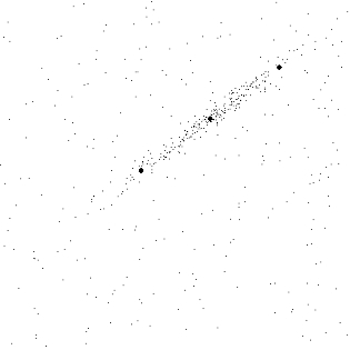
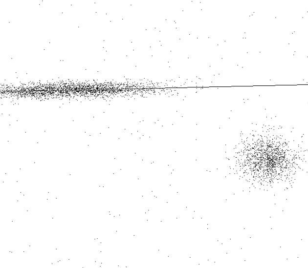
The standard deviation of the normal distribution along the straight line was one fourth of the length of the modeled segment (with this choice, approximately 95% of the points fall inside), and the length of the segment was taken equal to half the linear size of the square image (512 pixels). The dispersion ratio was 10.0, and the number of distribution points and the proportion of outlier noise varied. An example of this kind of distribution is shown in Figure 1.

In order to compare different algorithms, one must be able to evaluate how well a segment was found in each case. The subtlety lies in the fact that the considered algorithms are not looking for a segment, but a straight line. Therefore, we will take the “ideal” segment (A, B) and find a maximum of two distances from its ends to the experimentally found straight line. If we denote by Q (L, AB) the error in the parameters of the experimental line L, then this definition can be written as follows: Q (L, AB) = max (r (L, A), r (L, B)).

Fig. 1. Sample distribution with additive and outlier noise. Marks show the ends and center of the simulated segment.

Dependence of the error of the FHL method on the size of the smoothing window

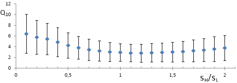
As mentioned above, regression using BPH involves smoothing. Obviously, the size of the smoothing window should have a significant impact on the quality of the algorithm. We investigate the dependence of the error of finding a straight line on the window size. For each size from a certain set, a series of one hundred images was generated, then a straight line was calculated for each and an error was recorded. The result obtained is shown in Figure 2 where the abscissa defines the ratio of the smoothing parameter s _H to the standard deviation of normal ( "transverse") sotstavlyayuschey s coordinate noise _L . The dots in the figure indicate the average errors, and the standard deviations are plotted up and down from them. You may notice that the result is best when s _Hclose to s _L , i.e. when the window size is not much different from the "thickness" of the segment.

Fig. 2. The dependence of the error of the Hough method on the size of the smoothing window.

Comparison with MNCs and its robust modifications

The most obvious, although incorrect (in our case) linear regression method is, of course, the least squares method (least squares), which for orthogonal regression coincides with the principal component method (PCA). At one time, for the case of outlier noise, it was doped up to “OLS with iterative recalculation of weights”, and all textbooks included variants with the Huber weight function and the biquadratic weight function [4].

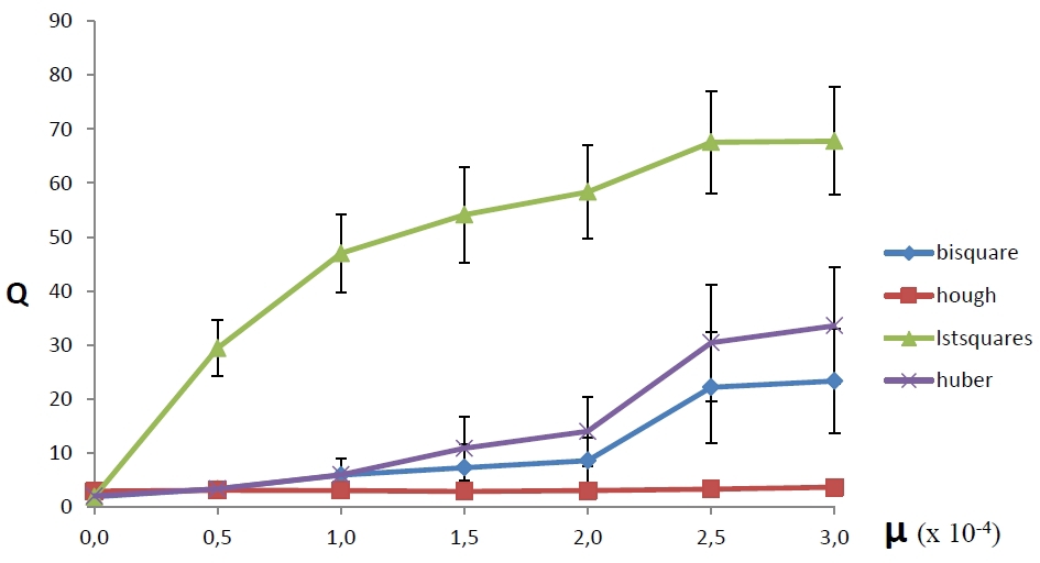
Compare the BPH method with a simple least-squares method, as well as with least-squares methods with recalculation of weights with both weight functions. We take the parameters of the functions, as theorists recommend: k _H = 1.345 for Huber and k _B = 4.685 for the biquadratic function.

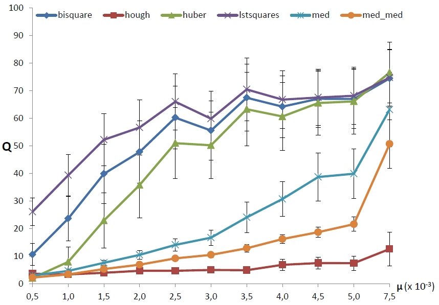
Figure 3 shows how the average error of each of the four methods depends on the density of the outlier noise µ - the ratio of the number of outlier noise points to the total number of pixels in the image (the outburst density is plotted along the abscissa axis, and the average error of the method is presented on the ordinate axis). Each measurement was carried out on a hundred different generated images. From the figure it is obvious that the method based on the use of the FHT turned out to be the most resistant to the addition of emission noise, although with a small number of emission points it is inferior to other methods in accuracy. In addition, this method turns out to be more stable, that is, it is less likely to make catastrophic mistakes (a quarter of the standard deviation of the error is postponed up and down from each point in the figure).

Fig. 3. The dependence of the average error on the density of the emission noise in the BPH and OLS methods.

Comparison with median methods

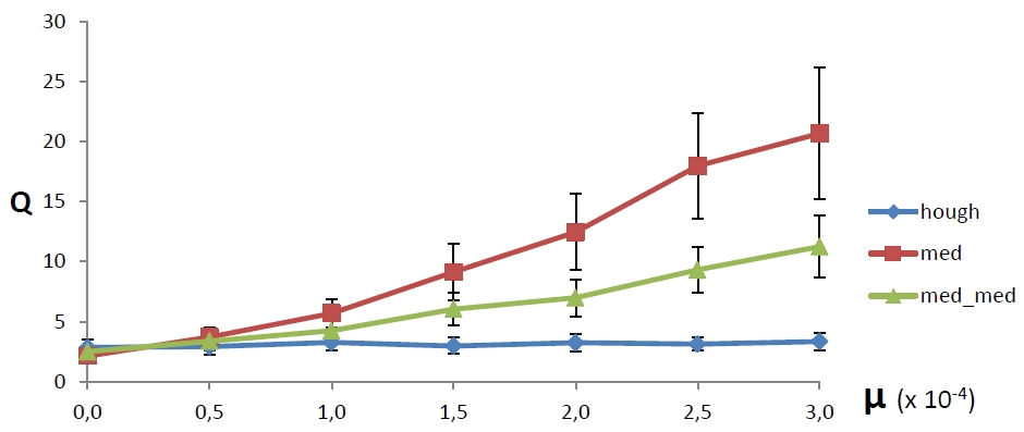
Surprisingly, they rarely talk about really good robust regression methods in universities. But we, dear reader, know about the magic Theil-Sen method [5], and therefore it would be dishonorable to limit ourselves to a comparison with robust OLS. In the classical Theil-Sen algorithm, the slope of the line is calculated as the median of the slopes of the lines drawn through all pairs of sample points. In addition, a modified version is used, in which, for each distribution point, the median of the slopes of all lines passing through this and some other distribution point is selected first, after which the median (“median of medians”) is selected from the obtained values. In both cases, the median among the values ​​{y _i - mx _i}, where m is the angular coefficient of the line found by the described methods.

Figure 4 shows a comparison now with these methods. As part of each series, a hundred experiments were still carried out, the designations also did not change. It can be seen that, in the considered range of ejection noise density, the average error of the BPH method is the smallest and does not grow, while the Theil-Sen methods have a proportional increase in error. It is also seen that the FHL method still has the smallest spread of error.

Fig. 4. The dependence of the average error on the density of the emission noise in the BPH and median methods.

Comparison of methods in the presence of structured noise

Of particular interest is the case when the outlier noise has its own spatial structure. For example, we add to the already considered types of noise a noise component uncorrelated with a signal with a circular two-dimensional normal distribution. An example of a combination of all three types of noise is shown in Figure 5. The straight line shows the perfect answer.

Fig. 5. An example of a segment noisy with additive, as well as uniform and structured emission noise.

Let us now look at the dependence of the error on the density of “round” structured noise with fixed parameters of outlier and additive noise. As before, one hundred images were generated for each density value. The results are shown in Figure 6. It is noticeable that the methods were divided into three groups, and surprisingly, classical robust methods differ little from OLS. It can be seen that the “breakdown” of all MNC methods occurs almost immediately, the median methods work stably with much larger data pollution, but they also stop working sooner or later, while the BPH method does not have a sharp breakdown at all.

Fig. 6. The dependence of the average error on the density of structured noise.

Discussion

Solving the linear regression problem using a combination of Gaussian smoothing and the Hough transform is resistant to both the additive coordinate and outlier noise. Comparison with other common robust methods showed that the proposed algorithm is more stable when the emission noise density is high enough. It should be noted at the same time that the method is applicable only in the small case (the BPH algorithm can be generalized to any dimension, but the amount of memory required to encode the task as an image of dimension higher than three is scary). In addition, even in the two-dimensional case, the use of the BPH will be disadvantageous if there are few points, and the required relative coordinate accuracy is high. This is due to the fact that for other methods, computational complexity depends on the number of points, and in BPH - on the number of discrete spaces. However, with a small number of points, it is possible to calculate the Hough transform by “brute force”. It would not seem like that, because we want to smooth the image first, but even Israel Moiseyevich Gelfand knew that Gaussian smoothing in a certain sense commutes with the Radon transform. Using this trick, the asymptotic behavior of the method in the approximation of a small number of points can be improved to O (n² ), however, n still indicates the linear size of the image, so it’s almost certainly too bad. But with a large number of points, the BPH method covers all other methods like a bull - a sheep. So it goes.

Literature

[1] DP Nikolaev, PP Nikolayev Linear color segmentation and its implementation, Computer Vision and Image Understanding. 2004, V.94 (Special issue on color for image indexing and retrieval), pp. 115-139
[2] L. Nolle. Application of computational intelligence for target tracking. In Proc. of 21st European Conference on Modeling and Simulation, 2007, pp. 289-293.
[3] DP Nikolaev, SM Karpenko, IP Nikolaev, PP Nikolaev. Hough transform: Underestimated Tool in Computer Vision Field. In Proc. of 22nd European Conference on Modeling and Simulation, 2008, pp. 238-243.
[4] PJ Rousseeuw, AM Leroy. Robust Regression and Outlier Detection. Wiley series in probability and statistics, 2003.
[5] Wilcox, R. Rand. Theil – Sen Estimator, Introduction to Robust Estimation and Hypothesis Testing, Academic Press, 2005, pp. 423-427.