Learn OpenGL. Lesson 5.10 - Screen Space Ambient Occlusion
- Transfer
- Tutorial

SSAO
The topic of background lighting was raised by us in a lesson on the basics of lighting , but only in passing. Let me remind you: the background component of lighting is essentially a constant value that is added to all calculations of the scene lighting to simulate the process of light scattering . In the real world, light undergoes many reflections with varying degrees of intensity, which leads to equally uneven illumination of indirectly illuminated portions of the scene. Obviously, flare with constant intensity is not very plausible.
One kind of approximate calculation of the shading of indirect lighting is the algorithm of background shading ( ambient occlusion, the AO), which simulates the attenuation of indirect lighting in the vicinity of corners, folds and other surface irregularities. Such elements, in general, are significantly overlapped by the adjacent geometry and therefore leave fewer rays of light to escape outside, obscuring these areas.
Below is a comparison of rendering without and using the AO algorithm. Pay attention to how the intensity of background lighting decreases in the vicinity of the corners of the walls and other sharp breaks in the surface:
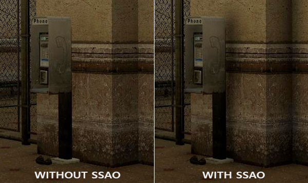
Although the effect is not very noticeable, the presence of the effect throughout the scene adds realism to it due to the additional illusion of depth created by small details of the self-shadowing effect.
Content
Part 1. Getting Started
Part 2. Basic lighting
Part 3. Download 3D models
Part 4. Advanced OpenGL Features
Part 5. Advanced Lighting
Part 6. PBR
- Opengl
- Window creation
- Hello window
- Hello triangle
- Shaders
- Textures
- Transformations
- Coordinate systems
- Camera
Part 2. Basic lighting
Part 3. Download 3D models
Part 4. Advanced OpenGL Features
- Depth test
- Stencil test
- Color mixing
- Clipping faces
- Frame buffer
- Cubic cards
- Advanced data handling
- Advanced GLSL
- Geometric shader
- Instancing
- Smoothing
Part 5. Advanced Lighting
- Advanced lighting. Blinn-Fong model.
- Gamma correction
- Shadow cards
- Omnidirectional shadow maps
- Normal mapping
- Parallax mapping
- HDR
- Bloom
- Deferred rendering
- SSAO
Part 6. PBR
It is worth noting that the algorithms for calculating AO are quite resource-intensive, since they require analysis of the surrounding geometry. In a naive implementation, it would be possible to simply emit a lot of rays at each point on the surface and determine the degree of its shadowing, but this approach very quickly reaches the resource-intensive limit acceptable for interactive applications. Fortunately, in 2007, Crytek has published a paper describing his own approach to the implementation of the algorithm of background shading in screen space ( Screen-Space the Ambient Occlusion, SSAO), which was used in the release version of the game Crysis. The approach calculated the degree of shadowing in the screen space, using only the current depth buffer instead of real data about the surrounding geometry. Such optimization radically accelerated the algorithm compared to the reference implementation and at the same time yielded mostly plausible results, which made this approach of approximate calculation of background shading a standard de facto industry.
The principle on which is based algorithm is quite simple: for each calculated fragment of the full-screen quad shading coefficient ( occlusion factor) based on the depth values of the surrounding fragments. The calculated shading coefficient is then used to reduce the intensity of background lighting (up to the complete exclusion). Obtaining a coefficient requires collecting depth data from a plurality of samples from the spherical region surrounding the fragment in question and comparing these depth values with the depth of the fragment in question. The number of samples having a depth greater than the current fragment directly determines the shading coefficient. Look at this diagram:
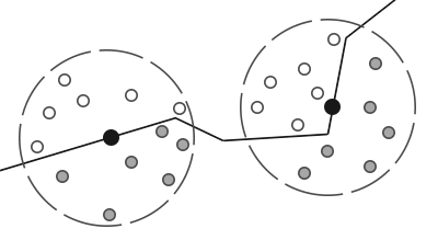
Here, each gray dot lies inside a certain geometric object, and therefore makes a contribution to the value of the shading coefficient. The more samples are inside the geometry of surrounding objects, the less will be the residual intensity of background shading in this area.
Obviously, the quality and realism of the effect directly depends on the number of samples taken. With a small number of samples, the accuracy of the algorithm decreases and leads to the appearance of a banding artifact ( banding) or “streaking” due to abrupt transitions between areas with very different shading factors. A large number of samples simply kills performance. Randomization of the core of the samples allows for somewhat similar results to slightly reduce the number of samples required. Reorientation by rotation to a random angle of a set of sample vectors is implied. However, introducing randomness immediately brings a new problem in the form of a noticeable noise pattern, which requires the use of blur filters to smooth the result. Below is an example of the algorithm (author - John Chapman ) and its typical problems: banding and noise pattern.

As can be seen, a noticeable banding due to the small number of samples is well removed by introducing randomization of the orientation of the samples.
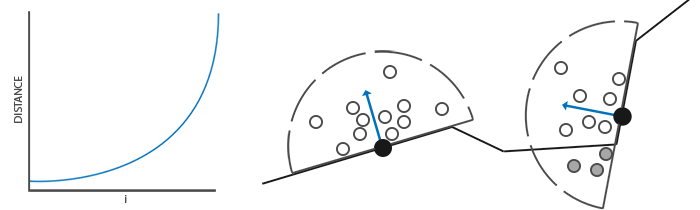
Crytek's specific SSAO implementation had a recognizable visual style. Since Crytek specialists used a spherical core of the sample, this affected even flat surfaces such as walls, making them shaded - because half of the volume of the core of the sample was submerged under the geometry. Below is a screenshot of a scene from Crysis shown in grayscale based on the value of the shading factor. Here the effect of "grayness" is clearly visible:

To avoid this effect, we will move from the spherical core of the sample to a hemisphere oriented along the normal to the surface:

Carrying out a sample of this hemisphere oriented along the normal ( normal-oriented hemisphere ), we do not have to be taken into account in calculating the coefficient of shading fragments lying beneath the surface of the adjacent surface. This approach removes unnecessary shading in, in general, gives more realistic results. This lesson will use the hemisphere approach and a bit more refined code from the brilliant SSAO lesson by John Chapman .
Raw data buffer
The process of calculating the shading factor in each fragment requires the availability of data about the surrounding geometry. Specifically, we need the following data:
- Position vector for each fragment;
- Normal vector for each fragment;
- Diffuse color for each fragment;
- The core of the sample
- A random rotation vector for each fragment used in reorienting the sample core.
Using data on the coordinates of the fragment in the species space, we can orient the hemisphere of the sample core along the normal vector specified in the species space for the current fragment. Then, the resulting core is used to make samples with various offsets from a texture that stores data on the coordinates of fragments. We make many samples in each fragment, and for each sample we make, we compare its depth value with the depth value from the fragment coordinate buffer to estimate the amount of shading. The resulting value is then used to limit the contribution of the background component in the final lighting calculation. Using a fragment-wise random rotation vector, we can significantly reduce the required number of samples to obtain a decent result, and then this will be demonstrated.

Since SSAO is an effect realized in the screen space, it is possible to perform a direct calculation by rendering a full-screen quad. But then we will not have data on the geometry of the scene. To get around this restriction, we will render all the necessary information in the texture, which will later be used in the SSAO shader to access geometric and other information about the scene. If you carefully followed these lessons, then you should already know in the described approach the appearance of the delayed shading algorithm. This is largely why the SSAO effect as a native appears in the render with deferred shading - after all, textures that store coordinates and normals are already available in the G-buffer.
In this lesson, the effect is implemented on top of a slightly simplified version of the code from the lesson on deferred lighting . If you have not yet familiarized yourself with the principles of deferred lighting, I strongly recommend that you turn to this lesson.
Since access to fragment information about coordinates and normals should already be available due to the G-buffer, the fragment shader of the geometry processing stage is quite simple:
#version 330 core
layout (location = 0) out vec4 gPosition;
layout (location = 1) out vec3 gNormal;
layout (location = 2) out vec4 gAlbedoSpec;
in vec2 TexCoords;
in vec3 FragPos;
in vec3 Normal;
void main()
{
    // положение фрагмента сохраняется в первой текстуре фреймбуфера
    gPosition = FragPos;
    // вектор нормали идет во вторую текстуру
    gNormal = normalize(Normal);
    // диффузный цвет фрагмента - в третью
    gAlbedoSpec.rgb = vec3(0.95);
}
Since the SSAO algorithm is an effect in the screen space, and the shading factor is calculated based on the visible area of the scene, it makes sense to carry out calculations in the view space. In this case, the FragPos variable obtained from the vertex shader stores the position exactly in the viewport. It is worth making sure that the coordinates and normals are stored in the G-buffer in the view space, since all further calculations will be carried out in it.
There is the possibility of restoring the position vector based on only a known fragment depth and a certain amount of mathematical magic, which is described, for example, in Matt Pettineo's blog . This, of course, requires a large calculation cost, but it eliminates the need to store position data in the G-buffer, which takes up a lot of video memory. However, for the sake of simplicity of the sample code, we will leave this approach for personal study.
The gPosition color buffer texture is configured as follows:
glGenTextures(1, &gPosition);
glBindTexture(GL_TEXTURE_2D, gPosition);
glTexImage2D(GL_TEXTURE_2D, 0, GL_RGB16F, SCR_WIDTH, SCR_HEIGHT, 0, GL_RGB, GL_FLOAT, NULL);
glTexParameteri(GL_TEXTURE_2D, GL_TEXTURE_MIN_FILTER, GL_NEAREST);
glTexParameteri(GL_TEXTURE_2D, GL_TEXTURE_MAG_FILTER, GL_NEAREST);
glTexParameteri(GL_TEXTURE_2D, GL_TEXTURE_WRAP_S, GL_CLAMP_TO_EDGE);
glTexParameteri(GL_TEXTURE_2D, GL_TEXTURE_WRAP_T, GL_CLAMP_TO_EDGE);
This texture stores the coordinates of fragments and can be used to obtain depth data for each point from the core of the samples. I note that the texture uses a floating-point data format - this will allow the coordinates of fragments not to be reduced to the interval [0., 1.]. Also pay attention to the repeat mode - GL_CLAMP_TO_EDGE is set . This is necessary to eliminate the possibility of not oversampling in the screen space on purpose. Going beyond the main interval of texture coordinates will give us incorrect position and depth data.
Next, we will engage in the formation of a hemispherical core of the samples and the creation of a method of random orientation.
Creating a normal-oriented hemisphere
So, the task is to create a set of sample points located inside a hemisphere oriented along the normal to the surface. Since the creation of the core samples for all possible directions of the normal computationally unattainable, we use the transition to the tangent space , where the normal is always represented as a vector in the direction of the positive half the Z .
Assuming the hemisphere radius to be a single process, the formation of a core of a sample of 64 points looks like this:
// случайные вещественные числа в интервале 0.0 - 1.0
std::uniform_real_distribution randomFloats(0.0, 1.0);
std::default_random_engine generator;
std::vector ssaoKernel;
for (unsigned int i = 0; i < 64; ++i)
{
    glm::vec3 sample(
        randomFloats(generator) * 2.0 - 1.0,
        randomFloats(generator) * 2.0 - 1.0,
        randomFloats(generator)
    );
    sample  = glm::normalize(sample);
    sample *= randomFloats(generator);
    float scale = (float)i / 64.0;
    ssaoKernel.push_back(sample);
}
Here we randomly select the x and y coordinates in the interval [-1., 1.], and the z coordinate in the interval [0., 1.] (if the interval is the same as for x and y , we would get a spherical core sampling). The resulting sample vectors will be limited to hemispheres, since the core of the sample will ultimately be oriented along the normal to the surface.
At the moment, all the sample points are randomly distributed inside the core, but for the sake of the quality of the effect, the samples lying closer to the origin of the kernel should make a greater contribution to the calculation of the shading coefficient. This can be realized by changing the distribution of the formed sample points by increasing their density near the origin. This task is easily accomplished using the acceleration interpolation function:
scale   = lerp(0.1f, 1.0f, scale * scale);
   sample *= scale;
   ssaoKernel.push_back(sample);
}
The lerp () function is defined as:
float lerp(float a, float b, float f)
{
    return a + f * (b - a);
}
Such a trick gives us a modified distribution, where most of the sample points lie near the origin of the kernel.
Each of the obtained sample vectors will be used to shift the coordinate of the fragment in the species space to obtain data on the surrounding geometry. To get decent results when working in the viewport, you may need an impressive number of samples, which will inevitably hit performance. However, the introduction of pseudo-random noise or rotation of the sample vectors in each processed fragment will significantly reduce the required number of samples with comparable quality.
Random rotation of the sample core
So, introducing randomness in the distribution of points in the core of the sample can significantly reduce the requirement for the number of these points to obtain a decent quality effect. It would be possible to create a random rotation vector for each fragment of the scene, but it is too expensive from memory. It’s more efficient to create a small texture containing a set of random rotation vectors, and then just use it with the GL_REPEAT repeat mode set .
Create a 4x4 array and fill it with random rotation vectors oriented along the normal vector in tangent space:
std::vector ssaoNoise;
for (unsigned int i = 0; i < 16; i++)
{
    glm::vec3 noise(
        randomFloats(generator) * 2.0 - 1.0,
        randomFloats(generator) * 2.0 - 1.0,
        0.0f);
    ssaoNoise.push_back(noise);
}
Since the core is aligned along the positive semiaxis Z in tangent space, we leave the z component equal to zero - this will ensure rotation only around the Z axis .
Next, create a 4x4 texture and fill it with our array of rotation vectors. Be sure to use GL_REPEAT replay mode to texture tiling:
unsigned int noiseTexture;
glGenTextures(1, &noiseTexture);
glBindTexture(GL_TEXTURE_2D, noiseTexture);
glTexImage2D(GL_TEXTURE_2D, 0, GL_RGB16F, 4, 4, 0, GL_RGB, GL_FLOAT, &ssaoNoise[0]);
glTexParameteri(GL_TEXTURE_2D, GL_TEXTURE_MIN_FILTER, GL_NEAREST);
glTexParameteri(GL_TEXTURE_2D, GL_TEXTURE_MAG_FILTER, GL_NEAREST);
glTexParameteri(GL_TEXTURE_2D, GL_TEXTURE_WRAP_S, GL_REPEAT);
glTexParameteri(GL_TEXTURE_2D, GL_TEXTURE_WRAP_T, GL_REPEAT);
Well, now we have all the data necessary for the direct implementation of the SSAO algorithm!
Shader SSAO
An effect shader will be executed for each fragment of a full-screen quad, calculating the shadowing coefficient in each of them. Since the results will be used in another rendering stage that creates the final lighting, we will need to create another framebuffer object to store the result of the shader:
unsigned int ssaoFBO;
glGenFramebuffers(1, &ssaoFBO);
glBindFramebuffer(GL_FRAMEBUFFER, ssaoFBO);
unsigned int ssaoColorBuffer;
glGenTextures(1, &ssaoColorBuffer);
glBindTexture(GL_TEXTURE_2D, ssaoColorBuffer);
glTexImage2D(GL_TEXTURE_2D, 0, GL_RED, SCR_WIDTH, SCR_HEIGHT, 0, GL_RGB, GL_FLOAT, NULL);
glTexParameteri(GL_TEXTURE_2D, GL_TEXTURE_MIN_FILTER, GL_NEAREST);
glTexParameteri(GL_TEXTURE_2D, GL_TEXTURE_MAG_FILTER, GL_NEAREST);
glFramebufferTexture2D(GL_FRAMEBUFFER, GL_COLOR_ATTACHMENT0, GL_TEXTURE_2D, ssaoColorBuffer, 0);
Since the result of the algorithm is the only real number within [0., 1.], for storage it will be enough to create a texture with the only available component. That is why GL_RED is set as the internal format for the color buffer .
In general, the SSAO stage rendering process looks something like this:
// проход геометрии: подготовка G-буфера
glBindFramebuffer(GL_FRAMEBUFFER, gBuffer);
    [...]
glBindFramebuffer(GL_FRAMEBUFFER, 0);
// используем G-буфер для создания текстуры с данными SSAO
glBindFramebuffer(GL_FRAMEBUFFER, ssaoFBO);
    glClear(GL_COLOR_BUFFER_BIT);
    glActiveTexture(GL_TEXTURE0);
    glBindTexture(GL_TEXTURE_2D, gPosition);
    glActiveTexture(GL_TEXTURE1);
    glBindTexture(GL_TEXTURE_2D, gNormal);
    glActiveTexture(GL_TEXTURE2);
    glBindTexture(GL_TEXTURE_2D, noiseTexture);
    shaderSSAO.use();
    SendKernelSamplesToShader();
    shaderSSAO.setMat4("projection", projection);
    RenderQuad();
glBindFramebuffer(GL_FRAMEBUFFER, 0);
// проход освещения: сведение итогового изображения
glClear(GL_COLOR_BUFFER_BIT | GL_DEPTH_BUFFER_BIT);
shaderLightingPass.use();
[...]
glActiveTexture(GL_TEXTURE3);
glBindTexture(GL_TEXTURE_2D, ssaoColorBuffer);
[...]
RenderQuad();
The shaderSSAO shader accepts the G-buffer textures it needs as input, as well as the noise texture and sample core:
#version 330 core
out float FragColor;
in vec2 TexCoords;
uniform sampler2D gPosition;
uniform sampler2D gNormal;
uniform sampler2D texNoise;
uniform vec3 samples[64];
uniform mat4 projection;
// тайлинг шумовой текстуры основан на отношении размера вьюпорта к размеру самой текстуры
// в примере вьюпорт имеет размер 1280x720
const vec2 noiseScale = vec2(1280.0/4.0, 720.0/4.0);
void main()
{
    [...]
}
Note the variable noiseScale . Our small texture with noise should be tiled over the entire surface of the screen, but since the TexCoords texture coordinates are within [0., 1.] this will not happen without our intervention. For these purposes, we calculate the factor for texture coordinates, which is found as the ratio of the screen size to the size of the noise texture:
vec3 fragPos   = texture(gPosition, TexCoords).xyz;
vec3 normal    = texture(gNormal, TexCoords).rgb;
vec3 randomVec = texture(texNoise, TexCoords * noiseScale).xyz;
Since when creating the texNoise noise texture we set the repeat mode to GL_REPEAT , now it will be repeated many times on the screen surface. With randomVec , fragPos, and normal values on hand , we can create a TBN transformation matrix from tangent to species space:
vec3 tangent   = normalize(randomVec - normal * dot(randomVec, normal));
vec3 bitangent = cross(normal, tangent);
mat3 TBN       = mat3(tangent, bitangent, normal);
Using the Gram-Schmidt process, we create an orthogonal basis randomly tilted in each fragment based on the random value randomVec . An important point: since in this case it doesn’t matter for us that the TBN matrix is exactly oriented along the surface of the triangle (as in the case with parallax mapping, approx. Per.), Then we do not need precalculated tangent and bi-tangent data.
Next, we go through the array of the sample core, translate each sample vector from the tangent space to the species space and get its sum with the current position of the fragment. Then we compare the depth value of the resulting amount with the depth value obtained by sampling from the corresponding G-buffer texture.
While it sounds confusing, let's go through the steps:
float occlusion = 0.0;
for(int i = 0; i < kernelSize; ++i)
{
    // получение координаты точки выборки
    vec3 sample = TBN * samples[i]; // переход от касательного в видовое пр-во
    sample = fragPos + sample * radius;
    [...]
}
Here, kernelSize and radius are variables that control the characteristics of the effect. In this case, they are 64 and 0.5, respectively. At each iteration, we translate the sample core vector into the species space. Next, we add to the obtained value of the displacement of the sample in the species space the value of the position of the fragment in the species space. In this case, the offset value is multiplied by the radius variable, which controls the radius of the core of the SSAO effect sample.
After these steps, we should convert the resulting sample vector into screen space, so that we can select from the G-buffer texture that stores the positions and depths of fragments using the obtained projected value. Since sampleis in the viewport, we need the projection matrix projection :
vec4 offset = vec4(sample, 1.0);
offset      = projection * offset;    // переход из видового  клиповое
offset.xyz /= offset.w;               // перспективное деление
offset.xyz  = offset.xyz * 0.5 + 0.5; // преобразование к интервалу [0., 1.]
After conversion to the clip space, we manually perform perspective division by simply dividing the xyz components by the w component. The resulting vector in normalized device coordinates ( NDC ) is translated into the interval of values [0., 1.] so that it can be used as texture coordinates:
float sampleDepth = texture(gPosition, offset.xy).z; We use the xy components of the sample vector to select from the texture the positions of the G-buffer. We get the depth value ( z components) corresponding to the sample vector when viewed from the observer's position (this is the first unshielded visible fragment). If at the same time the obtained sampling depth is greater than the stored depth, then we increase the shading coefficient:
occlusion += (sampleDepth >= sample.z + bias ? 1.0 : 0.0); Note the bias offset , which is added to the original fragment depth (set in the example to 0.025). This offset is not always required, but the presence of a variable allows you to control how the SSAO effect looks, and also, in certain situations, removes problems with ripples in shaded areas.
But this is not all, since such an implementation leads to noticeable artifacts. It manifests itself in cases when a fragment lying near the edge of a certain surface is considered. In such situations, when comparing the depths, the algorithm will inevitably capture the depths of surfaces, which can lie very far behind the considered one. In these places, the algorithm will erroneously greatly increase the degree of shadowing, which will create noticeable dark halos at the edges of objects. The artifact is treated by introducing an additional distance check (an example by John Chapman ):
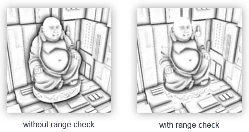
The check will limit the contribution to the shading coefficient only for depth values lying within the radius of the sample:
float rangeCheck = smoothstep(0.0, 1.0, radius / abs(fragPos.z - sampleDepth));
occlusion       += (sampleDepth >= sample.z + bias ? 1.0 : 0.0) * rangeCheck;
We also use the GLSL smoothstep () function , which implements smooth interpolation of the third parameter between the first and second. At the same time, returning 0 if the third parameter is less than or equal to the first, or 1 if the third parameter is greater than or equal to the second. If the depth difference is within radius , then its value will be smoothly smoothed in the interval [0., 1.] in accordance with this curve:

If we used clear boundaries in the conditions of checking depth, this would add artifacts in the form of sharp boundaries in those places where the values of the difference in depths are outside the limits of radius .
With the final touch, we normalize the value of the shading coefficient using the size of the sample core and record the result. We also invert the final value by subtracting it from unity, so that you can use the final value directly to modulate the background component of lighting without additional steps:
}
occlusion = 1.0 - (occlusion / kernelSize);
FragColor = occlusion;
For a scene with a lying nanosuit familiar to us, performing the SSAO shader gives the following texture:

As you can see, the effect of background shading creates a good illusion of depth. Only the output image of the shader already allows you to distinguish the details of the costume and make sure that it really lies on the floor, and does not levitate at some distance from it.
Nevertheless, the effect is far from ideal, since the noise pattern introduced by the texture of random rotation vectors is easily noticeable. To smooth the result of the SSAO calculation, we apply a blur filter.
Blur background shading
After building the result of SSAO and before the final mixing of lighting, it is necessary to blur the texture that stores data on the shading coefficient. To do this, we will have another framebuffer:
unsigned int ssaoBlurFBO, ssaoColorBufferBlur;
glGenFramebuffers(1, &ssaoBlurFBO);
glBindFramebuffer(GL_FRAMEBUFFER, ssaoBlurFBO);
glGenTextures(1, &ssaoColorBufferBlur);
glBindTexture(GL_TEXTURE_2D, ssaoColorBufferBlur);
glTexImage2D(GL_TEXTURE_2D, 0, GL_RED, SCR_WIDTH, SCR_HEIGHT, 0, GL_RGB, GL_FLOAT, NULL);
glTexParameteri(GL_TEXTURE_2D, GL_TEXTURE_MIN_FILTER, GL_NEAREST);
glTexParameteri(GL_TEXTURE_2D, GL_TEXTURE_MAG_FILTER, GL_NEAREST);
glFramebufferTexture2D(GL_FRAMEBUFFER, GL_COLOR_ATTACHMENT0, GL_TEXTURE_2D, ssaoColorBufferBlur, 0);
Tiling a noise texture in screen space provides well-defined randomness characteristics that you can use to your advantage when creating a blur filter:
#version 330 core
out float FragColor;
in vec2 TexCoords;
uniform sampler2D ssaoInput;
void main() {
    vec2 texelSize = 1.0 / vec2(textureSize(ssaoInput, 0));
    float result = 0.0;
    for (int x = -2; x < 2; ++x)
    {
        for (int y = -2; y < 2; ++y)
        {
            vec2 offset = vec2(float(x), float(y)) * texelSize;
            result += texture(ssaoInput, TexCoords + offset).r;
        }
    }
    FragColor = result / (4.0 * 4.0);
}
The shader simply transitions texels of the SSAO texture with an offset from -2 to +2, which corresponds to the actual size of the noise texture. The offset is equal to the exact size of one texel: the textureSize () function is used for calculation , which returns vec2 with the dimensions of the specified texture. T.O. The shader simply averages the results stored in the texture, which gives a quick and fairly effective blur:

In total, we have a texture with background shading data for each fragment on the screen - everything is ready for the stage of final image reduction!
Apply Background Shading
The step of applying the shading coefficient in the final calculation of lighting is surprisingly simple: for each fragment, it is enough to simply multiply the value of the background component of the light source by the shading coefficient from the prepared texture. You can take a ready-made shader with the Blinn-Fong model from the lesson on deferred shading and correct it a bit:
#version 330 core
out vec4 FragColor;
in vec2 TexCoords;
uniform sampler2D gPosition;
uniform sampler2D gNormal;
uniform sampler2D gAlbedo;
uniform sampler2D ssao;
struct Light {
    vec3 Position;
    vec3 Color;
    float Linear;
    float Quadratic;
    float Radius;
};
uniform Light light;
void main()
{
    // извлечение данных из G-буфера
    vec3 FragPos = texture(gPosition, TexCoords).rgb;
    vec3 Normal = texture(gNormal, TexCoords).rgb;
    vec3 Diffuse = texture(gAlbedo, TexCoords).rgb;
    float AmbientOcclusion = texture(ssao, TexCoords).r;
    // расчет модели Блинна-Фонга в видовом пространстве
    // здесь появляется новшество: учет расчитанного к-та затенения
    vec3 ambient = vec3(0.3 * Diffuse * AmbientOcclusion);
    vec3 lighting  = ambient;
    // положение наблюдателя всегда (0, 0, 0) в видовом пр-ве
    vec3 viewDir  = normalize(-FragPos);
    // диффузная составляющая
    vec3 lightDir = normalize(light.Position - FragPos);
    vec3 diffuse = max(dot(Normal, lightDir), 0.0) * Diffuse * light.Color;
    // зеркальная составляющая
    vec3 halfwayDir = normalize(lightDir + viewDir);
    float spec = pow(max(dot(Normal, halfwayDir), 0.0), 8.0);
    vec3 specular = light.Color * spec;
    // фоновая составляющая
    float dist = length(light.Position - FragPos);
    float attenuation = 1.0 / (1.0 + light.Linear * dist + light.Quadratic * dist * dist);
    diffuse  *= attenuation;
    specular *= attenuation;
    lighting += diffuse + specular;
    FragColor = vec4(lighting, 1.0);
}
There are only two major changes: the transition to calculations in the viewport and the multiplication of the background lighting component by the value of AmbientOcclusion . An example of a scene with a single blue point light:

The full source code is here .
The manifestation of the SSAO effect strongly depends on parameters such as kernelSize , radius and bias , often fine-tuning them is a matter of course for the artist to work out a particular location / scene. There are no “best” and universal combinations of parameters: for some scenes, a small radius of the sample core is good, while others benefit from the increased radius and number of samples. The example uses 64 sample points, which, frankly, is redundant, but you can always edit the code and see what happens with a smaller number of samples.
In addition to the listed uniforms that are responsible for setting the effect, there is the possibility to explicitly control the severity of the background shading effect. To do this, it is enough to raise the coefficient to a degree controlled by another uniform:
occlusion = 1.0 - (occlusion / kernelSize);
FragColor = pow(occlusion, power);
I advise you to spend some time on the game with the settings, as this will give a better understanding of the nature of the changes in the final picture.
To summarize, it is worth saying that although the visual effect of the use of SSAO is rather subtle, but in scenes with well-placed lighting, it undeniably adds a noticeable fraction of realism. Having such a tool in your arsenal is certainly valuable.
Additional Resources
- SSAO Tutorial : An excellent lesson article from John Chapman, on the basis of which the code for this lesson is built.
- Know your SSAO artifacts : A very valuable article lucidly showing not only the most pressing problems with SSAO quality, but also ways to solve them. Recommended reading.
- SSAO With Depth Reconstruction : Addendum to the main SSAO lesson by OGLDev regarding a commonly used technique for restoring fragment coordinates based on depth. The importance of this approach is due to the significant memory savings due to the lack of the need to store positions in the G-buffer. The approach is so universal, it applies to SSAO insofar as.
PS : We have a telegram conf for coordination of transfers. If you have a serious desire to help with the translation, then you are welcome!