How to properly measure disk performance
- Tutorial
abstract : the difference between current performance and theoretical performance; latency and IOPS, the concept of disk load independence; testing preparation; typical test parameters; practical copypaste howto.
Warning: many letters, long read.
A very common problem is an attempt to understand "how fast is the server?" Among all the tests, the most pathetic attempts to evaluate the performance of the disk subsystem. Here are the horrors I've seen in my life:
These are all completely wrong methods. Further I will analyze more subtle measurement errors, but with respect to these tests I can only say one thing - throw it out and do not use it.
bonnie ++ and iozone measure file system speed. Which depends on the cache, the thoughtfulness of the kernel, the success of the FS location on the disk, etc. Indirectly, you can say that if you got good results in iozone, then it is either a good cache, or a stupid set of parameters, or a really fast disk (guess which option you got). bonnie ++ is generally focused on file open / close operations. those. she does not particularly test disk performance.
dd without the direct option only shows the cache speed - no more. In some configurations, you can get linear speed without a cache higher than with a cache. In some you will receive hundreds of megabytes per second, with linear performance in units of megabytes.
With the direct option (iflag = direct for reading, oflag = direct for writing) dd only checks linear speed. Which is absolutely not equal to either the maximum speed (if we raid on many disks, then a raid in several streams can give more speed than in one), or real performance.
IOmeter is best of all, but it has problems working on linux. The 64-bit version does not correctly calculate the type of load and shows underestimated results (for those who do not believe, run it on ramdisk).
Spoiler: the correct utility for linux is fio. But it requires a very thoughtful test and an even more thoughtful analysis of the results. All that is below is just preparation of the theory and practical notes on working with fio.
(current VS maximum performance)
Now there will be even more boring letters. If someone is interested in the number of parrots on his favorite SSD'shka, laptop screw, etc. - see recipes at the end of the article.
All modern media except ramdisk have a very negative attitude to random write operations. For HDD there is no difference between writing or reading, it is important that the heads drive around the disk. For SSD, however, a random operation of reading nonsense, but writing with a small block leads to copy-on-write. The minimum recording size is 1-2 MB, they write 4kb. You need to read 2MB, replace them with 4KB and write back. As a result, for example, 400 requests per second for writing 4kb that turn into reading 800 Mb / s (!!!!) and writing them back goes to the SSD'shka. (For ramdisk, such a problem could be the same, but the intrigue is that the size of the "minimum block" for DDR is about 128 bytes, and the blocks in tests are usually 4k, so the DDR granularity is not important in tests of RAM disk performance) .
This post is not about the specifics of different media, so back to the general problem.
We cannot measure the entry in Mb / s. The important thing is how many head movements were, and how many random blocks we disturbed on the SSD. Those. The account goes to the number of IO operations, and the value of IO / s is called IOPS . Thus, when we measure a random load, we are talking about IOPS (sometimes wIOPS, rIOPS, for writing and reading, respectively). In large systems, they use the kIOPS value, (attention, always and everywhere, no 1024) 1kIOPS = 1000 IOPS.
And here, many fall into the trap of the first kind. They want to know how many IOPS the drive is giving out. Or a disk shelf. Or 200 server cabinets stuffed with disks under the covers.
It is important to distinguish between the number of operations performed (it is recorded that from 12:00:15 to 12:00:16 245790 disk operations were performed - that is, the load was 245kIOPS) and how much the system can perform maximum operations.
The number of operations performed is always known and easy to measure. But when we talk about disk operation, we talk about it in the future tense. "How many operations can the system perform?" - "what operations?" Different operations give a different load on the storage system. For example, if someone writes in random blocks of 1 MB, then he will receive much less iops than if he reads sequentially in blocks of 4 KB.
And if in the case of the load we are talking about how many requests were served "which came, they served," then in the case of planning, we want to know exactly which iops will be.
The drama is that no one knows what kind of requests will come. Little ones? Big ones? Contract? In a disagreement? Will they be read from the cache or will you have to go to the slowest place and pick out bytes from different halves of the disk?
I will not escalate the drama further, I will say that there is a simple answer:
As a result, we get numbers, each of which is incorrect. For example: 15kIOPS and 150 IOPS.
What will be the real system performance? This is determined only by how close the load will be to the good and bad end. (That is, the banal "life will show").
Most often they focus on the following indicators:
Well, about the block size. Traditionally, the test comes with a block size of 4k. Why? Because this is the standard block size that the OS operates on when saving the file. This is the size of the memory page and, in general, a Very Round Computer Number.
You need to understand that if the system processes 100 IOPS with a 4k block (worst), then it will process less with an 8k block (at least 50 IOPS, most likely around 70-80). Well, on the 1MB block we will see completely different numbers.
All? No, it was just an introduction. Everything that is written above is more or less well known. Nontrivial things start below.
First, we’ll look at the concept of “dependent IOPSs”. Imagine that our application works like this:
For convenience, we assume that the processing time is zero. If each read and write request will be serviced for 1ms, how many records per second can the application process? That's right, 500. And if we launch next to the second copy of the application? On any decent system, we get 1000. If we get significantly less than 1000, then we have reached the limit of system performance. If not, it means that the performance of an application with dependent IOPS is limited not by the storage performance, but by two parameters: latency and the level of IOPS dependency.
Let's start with latency. Latency - request execution time, delay before response. Usually use the value, "average delay." More advanced use the median.among all operations for a certain interval (most often for 1s). Latency is very difficult to measure. This is due to the fact that on any storage system, part of the requests is executed quickly, part is slow, and some can get into an extremely unpleasant situation and be serviced tens of times longer than the rest.
The intrigue is reinforced by the presence of a queue of requests, within which reordering of requests and their parallel execution can be carried out. A regular SATA drive has a queue depth (NCQ) of 31, and powerful storage systems can reach several thousand. (note that the actual length of the queue (the number of requests waiting to be completed) is rather a negative parameter, if there are a lot of requests in the queue, then they wait longer, i.e. slow down. Any person standing at rush hour in the supermarket will agree that the longer the queue, the shorter the service.
Latency directly affects the performance of a serial application, an example of which is given above. Higher latency - lower performance. At 5ms, the maximum number of requests is 200 pcs / s, at 20ms - 50. Moreover, if we have 100 requests processed in 1ms and 9 requests in 100ms, then in a second we will receive only 109 IOPS, with a median of 1ms and avg (average) at 10ms.
Hence the conclusion is rather difficult to understand: the type of load on performance affects not only whether it is “sequential” or “random”, but also how the applications using the disk are arranged.
Example: launching an application (typical desktop task) is almost 100% sequential. We read the application, read the list of necessary libraries, read each library in turn ... That is why on desktops they so passionately love SSDs - they have a microscopic delay (microsecond) for reading - of course, your favorite photoshop or blender starts in tenths of a second.
But, for example, the work of a loaded web server is almost parallel - each subsequent client is served independently of the neighboring one, i.e. latency affects only the service time of each client, but not the "maximum number of clients". And, we admit that 1ms, 10ms - for a web server anyway. (But it’s not “all the same” how many such parallel requests of 10ms can be sent).
Threshing. I think that desktop users are even more familiar with this phenomenon than sysadmins. A terrible crunch of the hard drive, unspeakable brakes, "nothing works and everything slows down."
As we begin to clog the disk queue (or storage, I repeat, in the context of the article there is no difference between them), latency begins to grow sharply. The disk runs to the limit, but there are more incoming calls than the speed of their service. Latency starts to grow rapidly, reaching horrific numbers of a few seconds (and this despite the fact that the application, for example, needs to do 100 operations to complete the work, which at a latency of 5 ms meant a half-second delay ...). This condition is called thrashing.
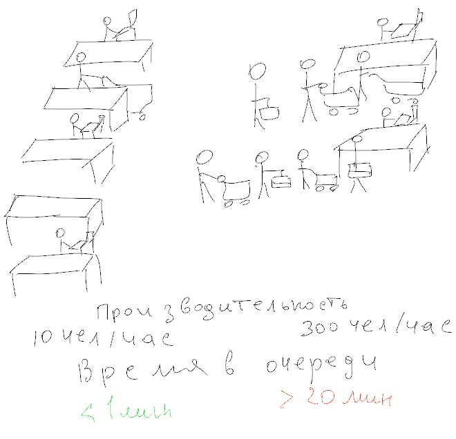
You will be surprised, but any disk or storage is capable of showing MORE IOPS in thrashing state than in normal loading. The reason is simple: if in normal mode the queue is most often emptyand the cashier is bored, waiting for customers , then in the trashing condition there is a constant service. (By the way, here's the explanation for why supermarkets like to arrange queues - in this case, the cashiers' productivity is maximum). True, customers do not like it much. And in good supermarkets they try to avoid such regimes. If you continue to raise the depth of the queue, then productivity will start to drop due to the queue being full and requests queuing to queue (yes, and the serial number with a ballpoint pen on your hand).
And here we are waiting for the next frequent (and very difficult to refute) error of those who measure disk performance.
They say, "My disk produces 180 IOPS, so if you take 10 disks, it will be as much as 1800 IOPS." (That's exactly what bad supermarkets think, planting fewer cashiers than necessary). At the same time, latency turns out to be transcendental - and "one cannot live like that."
A real performance test requires latency control, that is, the selection of such test parameters so that the latency remains below the agreed limit.
And here we are faced with a second problem: what is the limit? The theory cannot answer this question - this indicator is an indicator of the quality of service . In other words, everyone chooses for himself.
Personally, I conduct tests for myself so that the latency remains no more than 10ms. I consider this indicator to be the ceiling of storage performance. (at the same time, in my mind, I think for myself that the limit value after which lags begin to be felt is 20ms, but remember, about the example above from 900 to 1ms and 10 to 100ms, in which avg became 10ms? So, for this I reserve yourself + 10ms for random bursts).
We have already discussed the issue of dependent and independent IOPSs. The performance of dependent Iops is precisely controlled by latency, and we have already discussed this issue. But the performance in independent iops (i.e. with parallel load), what does it depend on?
The answer is from the imagination of the one who invented the disk or designed the storage. We can talk about the number of heads, spindles and parallel write queues in the SSD, but this is all speculation. From the point of view of practical use, we are interested in one question: HOW MUCH? How much can we run parallel load streams? (Do not forget about latency, because if we allow latency to go to heaven, the number of parallel threads will go there, however, not at that speed). So the question is: how many parallel threads can we execute at latency below a given threshold? Tests should answer this question.
Separately, we need to talk about the situation when the storage is connected to the host through a network using TCP. About TCP you need to write, write, write and write again. Suffice it to say that in Linux there are 12 different congestion control algorithms for the network that are designed for different situations. And there are about 20 kernel parameters, each of which can radically affect the output parrots (sorry, test results).
From the point of view of performance evaluation, we should simply accept this rule: for network attached storage, the test should be carried out from several hosts (servers) in parallel. Tests from a single server will not be a storage test, but will be an integrated test of the network, storage and the correct settings of the server itself.
The last question is the issue of shading the tire. What are you talking about? If we have ssd capable of delivering 400 MB / s, and we connect it via SATA / 300, then it is obvious that we will not see all the performance. Moreover, from the point of view of latency, the problem will begin to appear long before approaching 300MB / s, because each request (and the answer to it) will have to wait in line to slip through the bottleneck of the SATA cable.
But there are situations more fun. For example, if you have a shelf of drives connected via SAS / 300x4 (i.e. 4 SAS lines of 300MB each). It seems to be a lot. And if there are 24 disks in a shelf? 24 * 100 = 2400 MB / s, and we have only 1200 (300x4).
Moreover, tests on some (server!) Motherboards showed that built-in SATA controllers are often connected via PCIx4, which does not give the maximum possible speed for all 6 SATA connectors.
I repeat, the main problem in bus saturation is not eating out “under the ceiling” of the strip, but increasing latency as the bus loads.
Well, before practical advice, I’ll say about the famous tricks that can be found in industrial storages. First, if you read an empty disc, you will read it from nowhere. The systems are smart enough to feed you zeros from areas of the drive you never wrote to.
Secondly, in many systems, the first record is worse than the subsequent ones due to all sorts of snap shots, thin provision, deduplication, compression, late allocation, sparse placement, etc. In other words, it should be tested after the initial recording.
Thirdly, cache. If we are testing the worst case, then we need to know how the system will behave when the cache does not help. To do this, you need to take such a test size so that we are guaranteed to read / write "past the cache", that is, get out of the cache.
Write cache is a special story. He can save all write requests (sequential and random) and write them in comfort mode. The only worst case method is “cache trashing”, that is, sending write requests in such a volume and so long that the write cache stops writing and was forced to write data not in comfortable mode (combining adjacent areas), but discard random data by random writing. This can only be achieved by repeatedly exceeding the test area over the cache size.
Verdict - minimum x10 cache (frankly, the number is taken from the ceiling, I do not have an exact calculation mechanism).
Of course, the test should be without the participation of the local OS cache, that is, we need to run the test in a mode that would not use caching. In Linux, this is an O_DIRECT option when opening a file (or disk).
Total:
1) We are testing the worst case - 100% of the disk size, which is several times larger than the estimated cache size on the storage. For the desktop, this is just the “whole disk”, for industrial storages - a LUN or virtual machine disk size of 1TB or more. (Hehe, if you think that 64GB of RAM cache is a lot ...).
2) We conduct a test block in 4kb size.
3) We select the depth of parallelism of operations so that latency remains within reasonable limits.
At the output, we are interested in the parameters: IOPS number, latency, queue depth. If the test was run on several hosts, then the indicators are summarized (iops and queue depth), and for latency either avg or max is taken from the indicators for all hosts.
Here we move on to the practical part. There is a utility fio which allows us to achieve the result we need.
Normal fio mode involves the use of so-called job file, i.e. a config that describes exactly how the test looks. Examples of job files are given below, but for now we’ll discuss how fio works.
fio performs operations on the specified file (s). Instead of a file, a device may be indicated, i.e. we can exclude the file system from consideration. There are several test modes. We are interested in randwrite, randread and randrw. Unfortunately, randrw gives us dependent iops (reading comes after writing), so to get a completely independent test we have to do two parallel tasks - one for reading, the second for writing (randread, randwrite).
And we have to tell fio to do “preallocation”. (see above about the tricks of manufacturers). Next, we fix the block size (4k).
Another option is the disk access method. The fastest is libaio, which is what we will use.
Install fio: apt-get install fio (debian / ubntu). If anything, squeze doesn't have it yet.
The utility is very cunningly hidden, so it just doesn’t have a “home page”, only a git repository. Here is one of the mirrors: freecode.com/projects/fio
When testing a disk, you need to run it from root.
Launch: fio read.ini
Content read.ini
The task is to choose such iodepth so that avg.latency is less than 10ms.
(attention! Wrong drive letter - you will be left without data)
the most delicious part:
(attention! Mistake the drive letter - you will be left without data)
During the test, we see something like this:
In square brackets are the numbers of IOPS. But it's too early to rejoice - because we are interested in latency.
At the output (by Ctrl-C, or at the end) we get something like this:
^ C
fio: terminating on signal 2
We are interested in the following (in the minimum case):
read: iops = 3526 clat = 9063.18 (usec), i.e. 9ms.
write: iops = 2657 clat = 12028.23
Do not confuse slat and clat. slat is the time the request was sent (i.e., the performance of the Linux disk stack), and clat is the complete latency, that is, the latency we talked about. It is easy to see that reading is clearly more productive than writing, and I indicated excessive depth.
In the same example, I lower iodepth to 16/16 and get:
read 6548 iops, 2432.79usec = 2.4ms
write 5301 iops, 3005.13usec = 3ms
Obviously, the depth of 64 (32 + 32) turned out to be overkill, so much so that overall performance has even fallen. Depth 32 is much more suitable for testing.
Of course, everyone is already uncovering pi ... parrots. I give the values that I observed:
Warning: If you run this on virtual machines, then
a) if you charge for IOPS, it will be very tangible money.
b) If the hoster has poor storage, which relies only on a cache of several tens of gigabytes, then a test with a large disk (> 1TB) will lead to ... problems for the hoster and your hosting neighbors. Some hosts may be offended and ask you out.
c) Do not forget to zero the disk before the test (i.e. dd if = / dev / zero of = / dev / sdz bs = 2M oflag = direct)
Warning: many letters, long read.
Lyrics
A very common problem is an attempt to understand "how fast is the server?" Among all the tests, the most pathetic attempts to evaluate the performance of the disk subsystem. Here are the horrors I've seen in my life:
- A scientific publication in which cluster FS speed was evaluated using dd (and the file cache enabled, that is, without the direct option)
- using bonnie ++
- using iozone
- using cp bundles with runtime measurement
- using iometer with dynamo on 64-bit systems
These are all completely wrong methods. Further I will analyze more subtle measurement errors, but with respect to these tests I can only say one thing - throw it out and do not use it.
bonnie ++ and iozone measure file system speed. Which depends on the cache, the thoughtfulness of the kernel, the success of the FS location on the disk, etc. Indirectly, you can say that if you got good results in iozone, then it is either a good cache, or a stupid set of parameters, or a really fast disk (guess which option you got). bonnie ++ is generally focused on file open / close operations. those. she does not particularly test disk performance.
dd without the direct option only shows the cache speed - no more. In some configurations, you can get linear speed without a cache higher than with a cache. In some you will receive hundreds of megabytes per second, with linear performance in units of megabytes.
With the direct option (iflag = direct for reading, oflag = direct for writing) dd only checks linear speed. Which is absolutely not equal to either the maximum speed (if we raid on many disks, then a raid in several streams can give more speed than in one), or real performance.
IOmeter is best of all, but it has problems working on linux. The 64-bit version does not correctly calculate the type of load and shows underestimated results (for those who do not believe, run it on ramdisk).
Spoiler: the correct utility for linux is fio. But it requires a very thoughtful test and an even more thoughtful analysis of the results. All that is below is just preparation of the theory and practical notes on working with fio.
Formulation of the problem
(current VS maximum performance)
Now there will be even more boring letters. If someone is interested in the number of parrots on his favorite SSD'shka, laptop screw, etc. - see recipes at the end of the article.
All modern media except ramdisk have a very negative attitude to random write operations. For HDD there is no difference between writing or reading, it is important that the heads drive around the disk. For SSD, however, a random operation of reading nonsense, but writing with a small block leads to copy-on-write. The minimum recording size is 1-2 MB, they write 4kb. You need to read 2MB, replace them with 4KB and write back. As a result, for example, 400 requests per second for writing 4kb that turn into reading 800 Mb / s (!!!!) and writing them back goes to the SSD'shka. (For ramdisk, such a problem could be the same, but the intrigue is that the size of the "minimum block" for DDR is about 128 bytes, and the blocks in tests are usually 4k, so the DDR granularity is not important in tests of RAM disk performance) .
This post is not about the specifics of different media, so back to the general problem.
We cannot measure the entry in Mb / s. The important thing is how many head movements were, and how many random blocks we disturbed on the SSD. Those. The account goes to the number of IO operations, and the value of IO / s is called IOPS . Thus, when we measure a random load, we are talking about IOPS (sometimes wIOPS, rIOPS, for writing and reading, respectively). In large systems, they use the kIOPS value, (attention, always and everywhere, no 1024) 1kIOPS = 1000 IOPS.
And here, many fall into the trap of the first kind. They want to know how many IOPS the drive is giving out. Or a disk shelf. Or 200 server cabinets stuffed with disks under the covers.
It is important to distinguish between the number of operations performed (it is recorded that from 12:00:15 to 12:00:16 245790 disk operations were performed - that is, the load was 245kIOPS) and how much the system can perform maximum operations.
The number of operations performed is always known and easy to measure. But when we talk about disk operation, we talk about it in the future tense. "How many operations can the system perform?" - "what operations?" Different operations give a different load on the storage system. For example, if someone writes in random blocks of 1 MB, then he will receive much less iops than if he reads sequentially in blocks of 4 KB.
And if in the case of the load we are talking about how many requests were served "which came, they served," then in the case of planning, we want to know exactly which iops will be.
The drama is that no one knows what kind of requests will come. Little ones? Big ones? Contract? In a disagreement? Will they be read from the cache or will you have to go to the slowest place and pick out bytes from different halves of the disk?
I will not escalate the drama further, I will say that there is a simple answer:
- Test disk (storage / array) for best case (hit the cache, sequential operations)
- Disk test for worst case. Most often, such tests are planned with knowledge of the disk device. “Does it have 64MB cache?” And what if I make the size of the testing area 2GB? ” Does the hard drive read faster from the outside of the drive? And if I place the test area on the inside (closest to the spindle) area, so that the path traveled by the heads is more? Does he have read ahead prediction? And if I read in reverse order? Etc.
As a result, we get numbers, each of which is incorrect. For example: 15kIOPS and 150 IOPS.
What will be the real system performance? This is determined only by how close the load will be to the good and bad end. (That is, the banal "life will show").
Most often they focus on the following indicators:
- That best case is still best. Because you can optimize to such that the best case from the worst will hardly differ. This is bad (well, or we have such an awesome worst).
- At worst. Having it, we can say that the storage system will work faster than the figure obtained. Those. if we got 3000 IOPS, then we can safely use the system / disk in the load “up to 2000”.
Well, about the block size. Traditionally, the test comes with a block size of 4k. Why? Because this is the standard block size that the OS operates on when saving the file. This is the size of the memory page and, in general, a Very Round Computer Number.
You need to understand that if the system processes 100 IOPS with a 4k block (worst), then it will process less with an 8k block (at least 50 IOPS, most likely around 70-80). Well, on the 1MB block we will see completely different numbers.
All? No, it was just an introduction. Everything that is written above is more or less well known. Nontrivial things start below.
First, we’ll look at the concept of “dependent IOPSs”. Imagine that our application works like this:
- read record
- change record
- write back
For convenience, we assume that the processing time is zero. If each read and write request will be serviced for 1ms, how many records per second can the application process? That's right, 500. And if we launch next to the second copy of the application? On any decent system, we get 1000. If we get significantly less than 1000, then we have reached the limit of system performance. If not, it means that the performance of an application with dependent IOPS is limited not by the storage performance, but by two parameters: latency and the level of IOPS dependency.
Let's start with latency. Latency - request execution time, delay before response. Usually use the value, "average delay." More advanced use the median.among all operations for a certain interval (most often for 1s). Latency is very difficult to measure. This is due to the fact that on any storage system, part of the requests is executed quickly, part is slow, and some can get into an extremely unpleasant situation and be serviced tens of times longer than the rest.
The intrigue is reinforced by the presence of a queue of requests, within which reordering of requests and their parallel execution can be carried out. A regular SATA drive has a queue depth (NCQ) of 31, and powerful storage systems can reach several thousand. (note that the actual length of the queue (the number of requests waiting to be completed) is rather a negative parameter, if there are a lot of requests in the queue, then they wait longer, i.e. slow down. Any person standing at rush hour in the supermarket will agree that the longer the queue, the shorter the service.
Latency directly affects the performance of a serial application, an example of which is given above. Higher latency - lower performance. At 5ms, the maximum number of requests is 200 pcs / s, at 20ms - 50. Moreover, if we have 100 requests processed in 1ms and 9 requests in 100ms, then in a second we will receive only 109 IOPS, with a median of 1ms and avg (average) at 10ms.
Hence the conclusion is rather difficult to understand: the type of load on performance affects not only whether it is “sequential” or “random”, but also how the applications using the disk are arranged.
Example: launching an application (typical desktop task) is almost 100% sequential. We read the application, read the list of necessary libraries, read each library in turn ... That is why on desktops they so passionately love SSDs - they have a microscopic delay (microsecond) for reading - of course, your favorite photoshop or blender starts in tenths of a second.
But, for example, the work of a loaded web server is almost parallel - each subsequent client is served independently of the neighboring one, i.e. latency affects only the service time of each client, but not the "maximum number of clients". And, we admit that 1ms, 10ms - for a web server anyway. (But it’s not “all the same” how many such parallel requests of 10ms can be sent).
Threshing. I think that desktop users are even more familiar with this phenomenon than sysadmins. A terrible crunch of the hard drive, unspeakable brakes, "nothing works and everything slows down."
As we begin to clog the disk queue (or storage, I repeat, in the context of the article there is no difference between them), latency begins to grow sharply. The disk runs to the limit, but there are more incoming calls than the speed of their service. Latency starts to grow rapidly, reaching horrific numbers of a few seconds (and this despite the fact that the application, for example, needs to do 100 operations to complete the work, which at a latency of 5 ms meant a half-second delay ...). This condition is called thrashing.
You will be surprised, but any disk or storage is capable of showing MORE IOPS in thrashing state than in normal loading. The reason is simple: if in normal mode the queue is most often empty
And here we are waiting for the next frequent (and very difficult to refute) error of those who measure disk performance.
Latency control during test
They say, "My disk produces 180 IOPS, so if you take 10 disks, it will be as much as 1800 IOPS." (That's exactly what bad supermarkets think, planting fewer cashiers than necessary). At the same time, latency turns out to be transcendental - and "one cannot live like that."
A real performance test requires latency control, that is, the selection of such test parameters so that the latency remains below the agreed limit.
And here we are faced with a second problem: what is the limit? The theory cannot answer this question - this indicator is an indicator of the quality of service . In other words, everyone chooses for himself.
Personally, I conduct tests for myself so that the latency remains no more than 10ms. I consider this indicator to be the ceiling of storage performance. (at the same time, in my mind, I think for myself that the limit value after which lags begin to be felt is 20ms, but remember, about the example above from 900 to 1ms and 10 to 100ms, in which avg became 10ms? So, for this I reserve yourself + 10ms for random bursts).
Parallelism
We have already discussed the issue of dependent and independent IOPSs. The performance of dependent Iops is precisely controlled by latency, and we have already discussed this issue. But the performance in independent iops (i.e. with parallel load), what does it depend on?
The answer is from the imagination of the one who invented the disk or designed the storage. We can talk about the number of heads, spindles and parallel write queues in the SSD, but this is all speculation. From the point of view of practical use, we are interested in one question: HOW MUCH? How much can we run parallel load streams? (Do not forget about latency, because if we allow latency to go to heaven, the number of parallel threads will go there, however, not at that speed). So the question is: how many parallel threads can we execute at latency below a given threshold? Tests should answer this question.
SAN and NAS
Separately, we need to talk about the situation when the storage is connected to the host through a network using TCP. About TCP you need to write, write, write and write again. Suffice it to say that in Linux there are 12 different congestion control algorithms for the network that are designed for different situations. And there are about 20 kernel parameters, each of which can radically affect the output parrots (sorry, test results).
From the point of view of performance evaluation, we should simply accept this rule: for network attached storage, the test should be carried out from several hosts (servers) in parallel. Tests from a single server will not be a storage test, but will be an integrated test of the network, storage and the correct settings of the server itself.
bus saturation
The last question is the issue of shading the tire. What are you talking about? If we have ssd capable of delivering 400 MB / s, and we connect it via SATA / 300, then it is obvious that we will not see all the performance. Moreover, from the point of view of latency, the problem will begin to appear long before approaching 300MB / s, because each request (and the answer to it) will have to wait in line to slip through the bottleneck of the SATA cable.
But there are situations more fun. For example, if you have a shelf of drives connected via SAS / 300x4 (i.e. 4 SAS lines of 300MB each). It seems to be a lot. And if there are 24 disks in a shelf? 24 * 100 = 2400 MB / s, and we have only 1200 (300x4).
Moreover, tests on some (server!) Motherboards showed that built-in SATA controllers are often connected via PCIx4, which does not give the maximum possible speed for all 6 SATA connectors.
I repeat, the main problem in bus saturation is not eating out “under the ceiling” of the strip, but increasing latency as the bus loads.
Stunts manufacturers
Well, before practical advice, I’ll say about the famous tricks that can be found in industrial storages. First, if you read an empty disc, you will read it from nowhere. The systems are smart enough to feed you zeros from areas of the drive you never wrote to.
Secondly, in many systems, the first record is worse than the subsequent ones due to all sorts of snap shots, thin provision, deduplication, compression, late allocation, sparse placement, etc. In other words, it should be tested after the initial recording.
Thirdly, cache. If we are testing the worst case, then we need to know how the system will behave when the cache does not help. To do this, you need to take such a test size so that we are guaranteed to read / write "past the cache", that is, get out of the cache.
Write cache is a special story. He can save all write requests (sequential and random) and write them in comfort mode. The only worst case method is “cache trashing”, that is, sending write requests in such a volume and so long that the write cache stops writing and was forced to write data not in comfortable mode (combining adjacent areas), but discard random data by random writing. This can only be achieved by repeatedly exceeding the test area over the cache size.
Verdict - minimum x10 cache (frankly, the number is taken from the ceiling, I do not have an exact calculation mechanism).
OS local cache
Of course, the test should be without the participation of the local OS cache, that is, we need to run the test in a mode that would not use caching. In Linux, this is an O_DIRECT option when opening a file (or disk).
Test description
Total:
1) We are testing the worst case - 100% of the disk size, which is several times larger than the estimated cache size on the storage. For the desktop, this is just the “whole disk”, for industrial storages - a LUN or virtual machine disk size of 1TB or more. (Hehe, if you think that 64GB of RAM cache is a lot ...).
2) We conduct a test block in 4kb size.
3) We select the depth of parallelism of operations so that latency remains within reasonable limits.
At the output, we are interested in the parameters: IOPS number, latency, queue depth. If the test was run on several hosts, then the indicators are summarized (iops and queue depth), and for latency either avg or max is taken from the indicators for all hosts.
fio
Here we move on to the practical part. There is a utility fio which allows us to achieve the result we need.
Normal fio mode involves the use of so-called job file, i.e. a config that describes exactly how the test looks. Examples of job files are given below, but for now we’ll discuss how fio works.
fio performs operations on the specified file (s). Instead of a file, a device may be indicated, i.e. we can exclude the file system from consideration. There are several test modes. We are interested in randwrite, randread and randrw. Unfortunately, randrw gives us dependent iops (reading comes after writing), so to get a completely independent test we have to do two parallel tasks - one for reading, the second for writing (randread, randwrite).
And we have to tell fio to do “preallocation”. (see above about the tricks of manufacturers). Next, we fix the block size (4k).
Another option is the disk access method. The fastest is libaio, which is what we will use.
Practical recipes
Install fio: apt-get install fio (debian / ubntu). If anything, squeze doesn't have it yet.
The utility is very cunningly hidden, so it just doesn’t have a “home page”, only a git repository. Here is one of the mirrors: freecode.com/projects/fio
When testing a disk, you need to run it from root.
reading tests
Launch: fio read.ini
Content read.ini
[readtest]
blocksize = 4k
filename = / dev / sda
rw = randread
direct = 1
buffered = 0
ioengine = libaio
iodepth = 32
The task is to choose such iodepth so that avg.latency is less than 10ms.
Recording tests
(attention! Wrong drive letter - you will be left without data)
[writetest]
blocksize = 4k
filename = / dev / sdz
rw = randwrite
direct = 1
buffered = 0
ioengine = libaio
iodepth = 32
Hybrid tests
the most delicious part:
(attention! Mistake the drive letter - you will be left without data)
[readtest]
blocksize = 4k
filename = / dev / sdz
rw = randread
direct = 1
buffered = 0
ioengine = libaio
iodepth = 32
[writetest]
blocksize = 4k
filename = / dev / sdz
rw = randwrite
direct = 1
buffered = 0
ioengine = libaio
iodepth = 32
Output analysis
During the test, we see something like this:
Jobs: 2 (f = 2): [rw] [2.8% done] [13312K / 11001K / s] [3250/2686 iops] [eta 05m: 12s]
In square brackets are the numbers of IOPS. But it's too early to rejoice - because we are interested in latency.
At the output (by Ctrl-C, or at the end) we get something like this:
^ C
fio: terminating on signal 2
read: (groupid = 0, jobs = 1): err = 0: pid = 11048
  read: io = 126480KB, bw = 14107KB / s, iops = 3526, runt = 8966msec
    slat (usec): min = 3, max = 432, avg = 6.19, stdev = 6.72
    clat (usec): min = 387, max = 208677, avg = 9063.18, stdev = 22736.45
    bw (KB / s): min = 10416, max = 18176, per = 98.74%, avg = 13928.29, stdev = 2414.65
  cpu: usr = 1.56%, sys = 3.17%, ctx = 15636, majf = 0, minf = 57
  IO depths: 1 = 0.1%, 2 = 0.1%, 4 = 0.1%, 8 = 0.1%, 16 = 0.1%, 32 = 99.9%,> = 64 = 0.0%
     submit: 0 = 0.0%, 4 = 100.0%, 8 = 0.0%, 16 = 0.0%, 32 = 0.0%, 64 = 0.0%,> = 64 = 0.0%
     complete: 0 = 0.0%, 4 = 100.0%, 8 = 0.0%, 16 = 0.0%, 32 = 0.1%, 64 = 0.0%,> = 64 = 0.0%
     issued r / w: total = 31620/0, short = 0/0
     lat (usec): 500 = 0.07%, 750 = 0.99%, 1000 = 2.76%
     lat (msec): 2 = 16.55%, 4 = 35.21%, 10 = 35.47%, 20 = 3.68%, 50 = 0.76%
     lat (msec): 100 = 0.08%, 250 = 4.43%
write: (groupid = 0, jobs = 1): err = 0: pid = 11050
  write: io = 95280KB, bw = 10630KB / s, iops = 2657, runt = 8963msec
    slat (usec): min = 3, max = 907, avg = 7.60, stdev = 11.68
    clat (usec): min = 589, max = 162693, avg = 12028.23, stdev = 25166.31
    bw (KB / s): min = 6666, max = 14304, per = 100.47%, avg = 10679.50, stdev = 2141.46
  cpu: usr = 0.49%, sys = 3.57%, ctx = 12075, majf = 0, minf = 25
  IO depths: 1 = 0.1%, 2 = 0.1%, 4 = 0.1%, 8 = 0.1%, 16 = 0.1%, 32 = 99.9%,> = 64 = 0.0%
     submit: 0 = 0.0%, 4 = 100.0%, 8 = 0.0%, 16 = 0.0%, 32 = 0.0%, 64 = 0.0%,> = 64 = 0.0%
     complete: 0 = 0.0%, 4 = 100.0%, 8 = 0.0%, 16 = 0.0%, 32 = 0.1%, 64 = 0.0%,> = 64 = 0.0%
     issued r / w: total = 0/23820, short = 0/0
     lat (usec): 750 = 0.03%, 1000 = 0.37%
     lat (msec): 2 = 9.04%, 4 = 24.53%, 10 = 49.72%, 20 = 9.56%, 50 = 0.82%
     lat (msec): 100 = 0.07%, 250 = 5.87%
We are interested in the following (in the minimum case):
read: iops = 3526 clat = 9063.18 (usec), i.e. 9ms.
write: iops = 2657 clat = 12028.23
Do not confuse slat and clat. slat is the time the request was sent (i.e., the performance of the Linux disk stack), and clat is the complete latency, that is, the latency we talked about. It is easy to see that reading is clearly more productive than writing, and I indicated excessive depth.
In the same example, I lower iodepth to 16/16 and get:
read 6548 iops, 2432.79usec = 2.4ms
write 5301 iops, 3005.13usec = 3ms
Obviously, the depth of 64 (32 + 32) turned out to be overkill, so much so that overall performance has even fallen. Depth 32 is much more suitable for testing.
Performance Orientation
Of course, everyone is already uncovering pi ... parrots. I give the values that I observed:
- RAMDISK (rbd) - ~ 200kIOPS / 0.1ms (iodepth = 2)
- SSD (intel 320th series) - 40k IOPS read (0.8ms); about 800 IOPS per record (after a long testing time)
- SAS disk (15k RPM) - 180 IOPS, 9ms
- SATA drive (7.2, WD RE) - 100 IOPS, 12ms
- SATA WD Raptor - 140 IOPS, 12mc
- SATA WD Green - 40 IOPS, and I was not able to achieve latency <20 even with iodepth = 1
Warning: If you run this on virtual machines, then
a) if you charge for IOPS, it will be very tangible money.
b) If the hoster has poor storage, which relies only on a cache of several tens of gigabytes, then a test with a large disk (> 1TB) will lead to ... problems for the hoster and your hosting neighbors. Some hosts may be offended and ask you out.
c) Do not forget to zero the disk before the test (i.e. dd if = / dev / zero of = / dev / sdz bs = 2M oflag = direct)