Development of proteins in the cloud using Python and Transcriptic or How to create any protein for $ 360
- Transfer
What if you have an idea for a cool, healthy protein, and you want to get it in reality? For example, would you like to create a vaccine against H. pylori (like the Slovenian team at iGEM 2008 ) by creating a hybrid protein that combines E. coli flagellin fragments that stimulate the immune response with the usual H. pylori flagellin ?
 Design of the hybrid flagellin vaccine against H. pylori presented by the Slovenian team at iGEM 2008
Surprisingly, we are very close to creating any protein we want without leaving the Jupyter notebook thanks to the latest developments in genomics, synthetic biology, and more recently - in cloud labs.
In this article, I will show Python code from the idea of a protein to its expression in a bacterial cell, without touching a pipette or talking to anyone. The total cost will be only a few hundred dollars! Using the terminology of Vijaya Pande from A16Z , this is Biology 2.0.
More specifically, in the article, the Python code of the cloud lab does the following:
First, the general Python settings that are needed for any Jupyter notepad. We import some useful Python modules and create some utility functions, mainly for data visualization.
Like AWS or any computing cloud, the cloud lab has molecular biology equipment, as well as robots that it leases over the Internet. You can issue instructions to your robots by clicking a few buttons on the interface or by writing code that programs them yourself. It is not necessary to write your own protocols, as I will do here, a significant part of molecular biology is standard routine tasks, so it is usually better to rely on a reliable alien protocol that showed good interaction with robots.
Recently, a number of companies with cloud labs have appeared: Transcriptic , Autodesk Wet Lab Accelerator (beta, and built on the basis of Transcriptic), Arcturus BioCloud (beta),Emerald Cloud Lab (beta), Synthego (not yet launched). There are even companies built on top of cloud labs such as Desktop Genetics , which specializes in CRISPR. Scientific articles about the use of cloud labs in real science are starting to appear .
At the time of this writing, only Transcriptic is in the public domain, so we will use it. As I understand it, most of the Transcriptic business is built on automating common protocols, and writing your own protocols in Python (as I will do in this article) is less common.
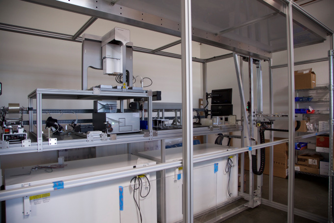
Transcriptic “working cell” with refrigerators at the bottom and various laboratory equipment at the stand
I will give Transcriptic robots instructions onauto protocol . Autoprotocol is a JSON-based language for writing protocols for laboratory robots (and humans, as it were). Autoprotocol is mainly made on this Python library . The language was originally created and is still supported by Transcriptic, but, as I understand it, it is completely open. There is good documentation .
An interesting idea is that on the auto-protocol you can write instructions for people in remote laboratories - say, in China or India - and potentially get some advantages from using both people (their judgment) and robots (lack of judgment). We need to mention protocols.io here , this is an attempt to standardize protocols to improve reproducibility, but for humans, not robots.
Autoprotocol fragment example
In addition to importing standard libraries, I will need some specific molecular biological utilities. This code is mainly for auto-protocol and Transcriptic.
The concept of “dead volume” is often found in code. This means the last drop of liquid that Transcriptic robots cannot take with a pipette from the tubes (because they cannot see it!). You have to spend a lot of time to make sure that the flasks have enough material.
Despite its connection with modern synthetic biology, DNA synthesis is a fairly old technology. For decades, we have been able to make oligonucleotides (that is, DNA sequences up to 200 bases). However, it was always expensive, and chemistry never allowed long DNA sequences. Recently, it has become possible at a reasonable price to synthesize whole genes (up to thousands of bases). This achievement truly opens the era of “synthetic biology”.
The company Synthetic Genomics Craig Venter's synthetic biology has advanced furthest, synthesizing the whole organism - more than a million bases in length. As the length of the DNA increases, the problem is no longer synthesis, but assembly (i.e., stitching together synthesized DNA sequences). With each assembly, you can double the DNA length (or more), so after a dozen or so iterations, you get a rather long molecule ! The distinction between synthesis and assembly should soon become clear to the end user.
The price of DNA synthesis is falling pretty fast, from over $ 0.30 a year ago two to about $ 0.10 today, but it is developing more like bacteria than processors. In contrast, DNA sequencing prices are falling faster than Moore’s law. A target of $ 0.02 per base is set as an inflection point where you can replace a lot of time-consuming DNA manipulations with simple synthesis. For example, at this price, you can synthesize a whole 3kb plasmid for $ 60 and skip a bunch of molecular biology. I hope we will achieve this in a couple of years.
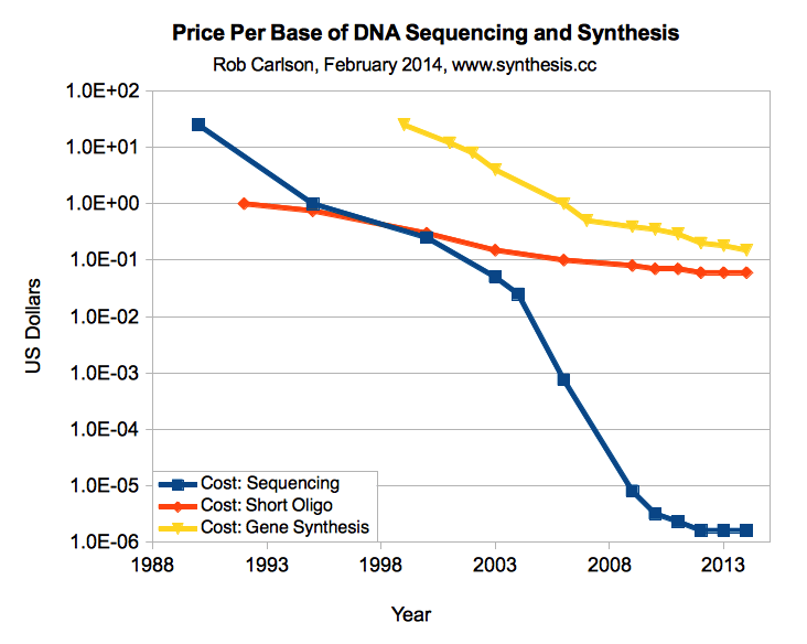
DNA synthesis prices compared to DNA sequencing prices, price for 1 base (Carlson, 2014)
There are several large companies in the field of DNA synthesis: IDT is the largest producer of oligonucleotides, and can also produce longer (up to 2kb) “gene fragments” ( gBlocks ). Gen9 , Twist, and DNA 2.0 typically specialize in longer DNA sequences - these are gene synthesis companies. There are also some interesting new companies, such as Cambrian Genomics and Genesis DNA , that are working on next-generation synthesis methods.
Other companies such as Amyris , Zymergen and Ginkgo Bioworks, use the DNA synthesized by these companies to work at the body level. Synthetic Genomics does this too, but it synthesizes DNA itself.
Ginkgo recently struck a deal with Twist to make 100 million bases: the largest deal I've seen. This proves that we live in the future, Twist even advertised a promotional code on Twitter: when you buy 10 million DNA bases (almost the entire yeast genome!), You get another 10 million for free.
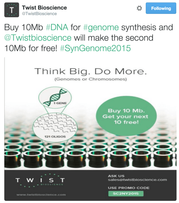
Twitter Twist Niche Offer
In this experiment, we synthesize a DNA sequence for a simple, green fluorescent protein (GFP). The GFP protein was first found in a jellyfish that fluoresces under ultraviolet light. This is an extremely useful protein because it is easy to detect its expression simply by measuring fluorescence. There are GFP options that produce yellow, red, orange, and other colors.
It is interesting to see how various mutations affect the color of a protein, and this is a potentially interesting machine learning problem. More recently, you would have to spend a lot of time in the laboratory for this, but now I will show you that it is (almost) as easy as editing a text file!
Technically, my GFP is a Super Folder Option (sfGFP) with some mutations to improve quality.
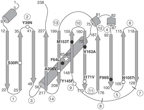
In superfolder-GFP (sfGFP), some mutations give it certain useful properties.
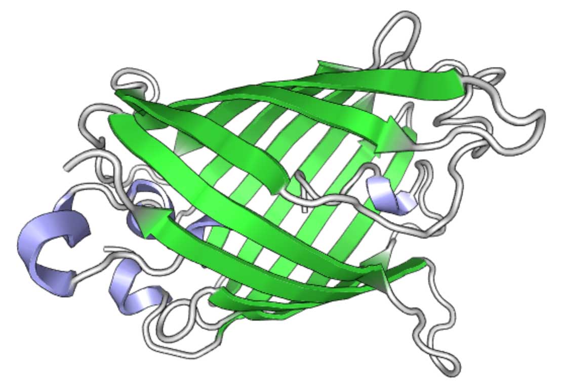
GFP structure (visualized using PV )
I was fortunate enough to get into Twist's alpha testing program, so I used their DNA synthesis service (they kindly placed my tiny order - thanks, Twist!). This is a new company in our field, with a new simplified synthesis process. Their prices are around $ 0.10 per base or lower , but they are still in beta , and the alpha program in which I participated was closed. Twist raised about $ 150 million, so their technology is lively.
I sent my DNA sequence to Twist as an Excel spreadsheet (there is no API yet, but I guess it will be soon), and they sent the synthesized DNA directly to my box in the Transcriptic laboratory (I also used IDT for synthesis, but they did not send DNA right in Transcriptic, which spoils the fun a bit).
Obviously, this process has not yet become a typical use case and requires some support, but it worked, so that the entire pipeline remains virtual. Without this, I probably would need access to the laboratory - many companies will not send DNA or reagents to their home address.
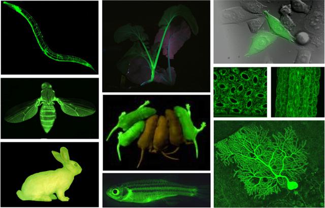
GFP is harmless, so any kind is highlighted
To express this protein in bacteria, the gene needs to live somewhere, otherwise the synthetic DNA encoding the gene simply degrades instantly. As a rule, in molecular biology we use a plasmid, a piece of round DNA that lives outside the bacterial genome and expresses proteins. Plasmids are a convenient way for bacteria to share useful, stand-alone functional modules, such as antibiotic resistance. There can be hundreds of plasmids in a cell.
Widely used terminology is that a plasmid is a vector , and synthetic DNA is an insertion (insertion). So, here we are trying to clone the insertion into a vector, and then transform the bacteria using the vector.
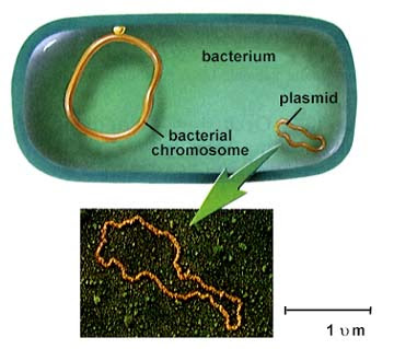
Bacterial genome and plasmid (not to scale!) ( Wikipedia )
I chose a fairly standard plasmid in the pUC19 series . This plasmid is very often used, and since it is available as part of the standard Transcriptic inventory, we do not need to send anything to them.
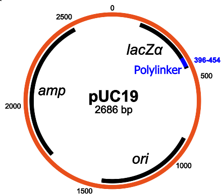
Structure of pUC19: the main components are the gene for resistance to ampicillin, lacZα, MCS / polylinker and the origin of replication (Wikipedia)
pUC19 has a nice function: since it contains the lacZα gene, you can use the blue-white selection method and see which colonies are successfully The insertion has passed. Two chemicals are needed: IPTG and X-gal , and the circuit works as follows:
Blue-white selection shows where lacZα expression was deactivated ( Wikipedia )
The openwetware documentation says:
It is easy to obtain the DNA sequence for sfGFP by taking the protein sequence and encoding it with codons suitable for the host organism (here, E. coli ). This is a medium-sized protein with 236 amino acids, so at 10 cents DNA synthesis costs about $ 70 per base .
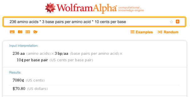
Wolfram Alpha, calculation of the cost of synthesis
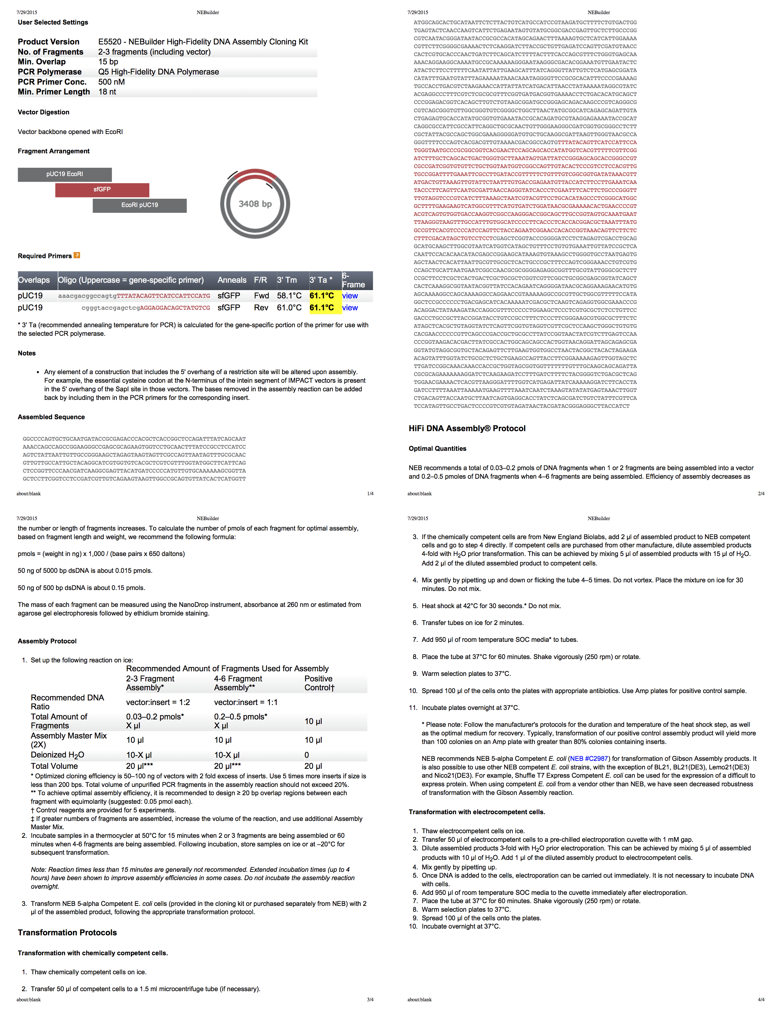
The first 12 bases of our sfGFP are the Shine-Delgarno sequence , which I added myself, which theoretically should increase expression (AGGAGGACAGCT, then ATG ( start codon ) launches the protein). According to a computing tool developed by Salis Lab ( lecture slides), we can expect medium to high expression of our protein (translation initiation rate of 10,000 “arbitrary units”).
First, I check that the pUC19 sequence that I downloaded from the NEB has the correct length and it includes the expected polylinker .
We do some basic QCs to make sure that EcoRI and BamHI are present in pUC19 only once (the following restriction enzymes are available in the default Transcriptic inventory: PstI , PvuII , EcoRI , BamHI , BbsI , BsmBI ).
Now we look at the lacZα sequence and verify that there is nothing unexpected. For example, it should begin with Met and end with a stop codon. It is also easy to confirm that this is the full 324bp lacZα ORF by loading the pUC19 sequence into the free snapgene viewer .
Assembling DNA simply means crosslinking fragments. Usually you collect several DNA fragments into a longer segment, and then clone it into a plasmid or genome. In this experiment, I want to clone one segment of DNA into the pUC19 plasmid below the lac promoter for expression in E. coli .
There are many cloning methods (e.g. NEB , openwetware , addgene ). Here I will use the Gibson assembly ( developed by Daniel Gibsonat Synthetic Genomics in 2009), which is not necessarily the cheapest method, but simple and flexible. You just need to put the DNA that you want to collect (with the appropriate overlap) in a test tube with the Gibson Assembly Master Mix, and it will assemble itself!
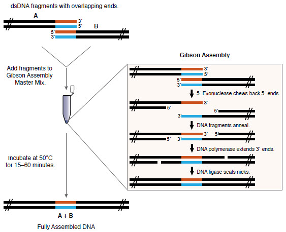
Gibson Assembly Review ( NEB )
We start with 100 ng of synthetic DNA in 10 μl of liquid. This equals 0.21 picomoles of DNA or a concentration of 10 ng / μl.
According to the NEB assembly protocol , this is enough source material:
NEBuilder from the company Biolab - it really is a great tool for creating a protocol Gibson assembly. It even generates you a comprehensive four-page PDF with all the information. Using this tool, we develop a protocol for cutting pUC19 with EcoRI, and then use PCR [PCR, polymerase chain reaction allows to achieve a significant increase in small concentrations of certain DNA fragments in biological material - approx. per.] to add fragments of the appropriate size to the insertion.
The experiment consists of four stages:
Gibson assembly depends on the DNA sequence that you collect, having some overlapping sequence (see NEB protocol with detailed instructions above). In addition to simple amplification, PCR also allows you to add a flanking DNA sequence by simply including an additional sequence in the primers (can also be cloned using only OE-PCR ).
We synthesize primers according to the NEB protocol above. I tried the Quickstart protocol on the Transcriptic site, but there is still an auto- protocol command. Transcriptic itself does not synthesize oligonucleotides, so after 1-2 days of waiting, these primers magically appear in my inventory (note that the gene-specific part of the primers is indicated in upper case below, but these are just cosmetic things).
You can analyze the properties of these primers using the IDT OligoAnalyzer . when debugging a PCR experiment, it is useful to know the melting points and the likelihood of a side effect of primer dimer , although the NEB protocol will almost certainly select primers with good properties.
I went through many iterations of PCR before getting satisfactory results, including experiments with several different brands of PCR blends. Since each of these iterations can take several days (depending on the length of the queue to the laboratory), it is worth spending time on debugging in advance: this saves a lot of time in the long run. As the power of the cloud lab increases, this problem should become less acute. However, it is unlikely that your first protocol will succeed - there are too many variables.
In the gel, you can evaluate the correct size of the product after increasing the concentration (the position of the strip in the gel) and the correct amount (dark strip). The gel has a ladder corresponding to various lengths and amounts of DNA that can be used for comparison.
In the gel photograph below, the bands D1, E1, F1 contain, respectively, 2 μl, 4 μl and 8 μl of the amplified product. I can estimate the amount of DNA in each lane compared to the DNA in the ladder (50 ng DNA per lane in the ladder). I think the results look very clean.
I tried to use GelEval for image analysis and concentration estimation, and quite successfully, although I'm not sure if this is much more accurate than the more naive method. However, small changes in the location and size of the bands led to large changes in the estimation of the amount of DNA. My best estimate of the amount of DNA in my amplified product using GelEval is 40 ng / μl.
Assuming we are limited by the amount of primer in the mixture and not by the amount of dNTP or enzyme, since I have 12.5 pmol of each primer, this means a theoretical maximum of 6 μg of 740bp DNA in 25 μl. Since my estimate of the total amount of DNA using GelEval is 40 ng x 25 μl (1 μg or 2 pmol), these results are very reasonable and close to what I should expect under ideal conditions.
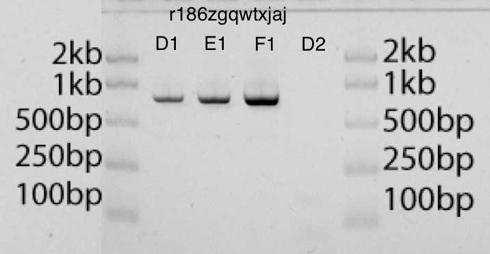
Гель-электрофорез EcoRI-среза pUC19, различные концентрации (D1, E1, F1), плюс контроль (D2)
Transcriptic recently started providing interesting and useful diagnostic data from its robots. At the time of writing, they are not available for download, so for now I only have an image of temperatures during thermal cycling.
Data looks good, without unexpected peaks or troughs. A total of 35 PCR cycles, but some of these cycles are carried out at very high temperatures as part of the PCR touchdown . In my previous attempts to amplify this segment - of which there were several! - there were problems with the hybridization of the primers, so here the PCR works for a lot of time at high temperatures, which should increase the accuracy.
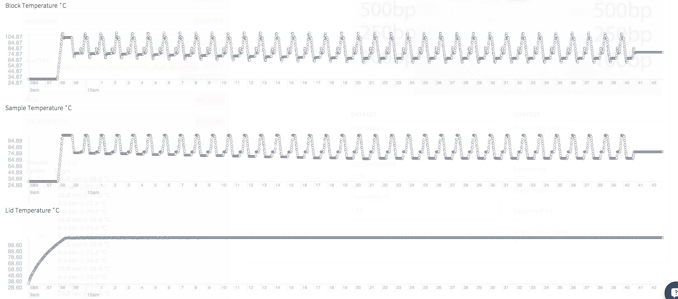
Thermocyclic diagnostics for touchdown PCR: block, sample and cover temperatures for 35 cycles and 42 minutes
To insert our sfGFP DNA into pUC19, you first need to cut the plasmid. Following the NEB protocol, I do this using the EcoRI restriction enzyme . There are reagents that I need in the standard Transcriptic inventory: this is NEB EcoRI and 10x CutSmart buffer , as well as NEB pUC19 plasmid .
For information, below are the prices from their inventory. In fact, I pay only part of the price, since Transcriptic takes payment for the amount actually consumed:
I followed the NEB protocol as much as possible:
I conducted this experiment twice under slightly different conditions and with gels of different sizes, but the results are almost identical. I like both gels.
Initially, I did not allocate enough space for the “dead” volume (in test tubes of 1.5 ml, the dead volume is 15 μl!). I think this explains the difference between D1 and E1 (the two bands should be identical). The dead volume problem is easy to solve by creating the proper working supply of diluted EcoRI at the start of the protocol.
Despite this error, in both gels the D1 and E1 bands have strong bands in the correct position of 2.6kb. On band D2, an uncut plasmid: as expected, it is not visible in one gel and barely visible in another.
Two gel photos look quite different. This is partly due to the fact that this step Transcriptic has not yet automated.
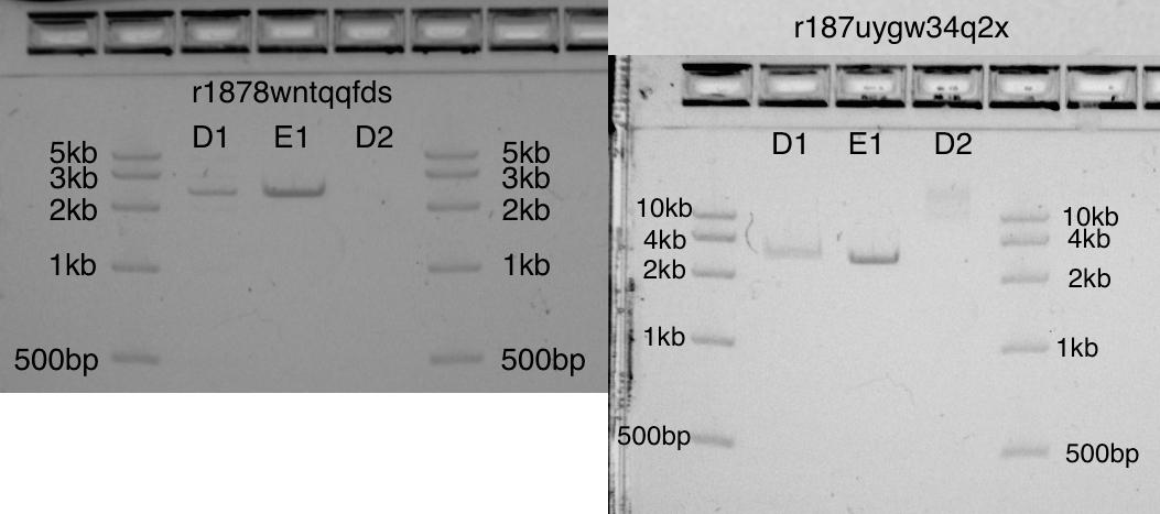
Two gels showing cut pUC19 (2.6kb) in bands D1 and E1, and uncut pUC19 in D2
The easiest way to check if my assembly works using the Gibson method is to collect the insertion and plasmid, then use standard M13 primers (which flank the insertion) to amplify part of the plasmid and inserted DNA and run qPCR and gel to make sure that the amplification worked. You can also run a sequencing reaction to confirm that everything is inserted as expected, but I decided to leave it for later.
If the Gibson assembly does not work, then the amplification of M13 does not work because the plasmid was cut between two M13 sequences.
I can access qPCR data in JSON format through the Transcriptic API. This feature is not well documented , but can be extremely useful. The APIs even give you access to some diagnostic data from robots, which can help with debugging.
First, we request launch data:
Then we specify this id to get the qPCR "post-processing" data:
Here are the Ct values (cycle threshold) for each tube. Ct is simply the point at which fluorescence exceeds a certain value. She says roughly how much DNA is there at the moment (and therefore, roughly where we started).
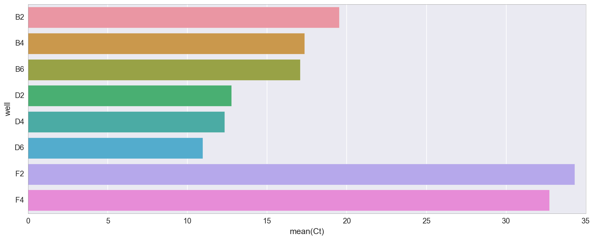
As you can see, amplification primarily occurs in test tubes D2 / 4/6 (where the DNA from my Gibson assembly is “v3”), then B2 / 4/6 (Gibson assembly is “v1”). The differences between v1 and v3 are basically that v3 DNA is diluted 4X according to the NEB protocol, but both options should work. There is some amplification after cycle 30 in control tubes (F2, F4) lacking a DNA template, but this is not uncommon, as they include a lot of primer DNA.
I can also plot the qPCR amplification curve to see the dynamics of amplification.
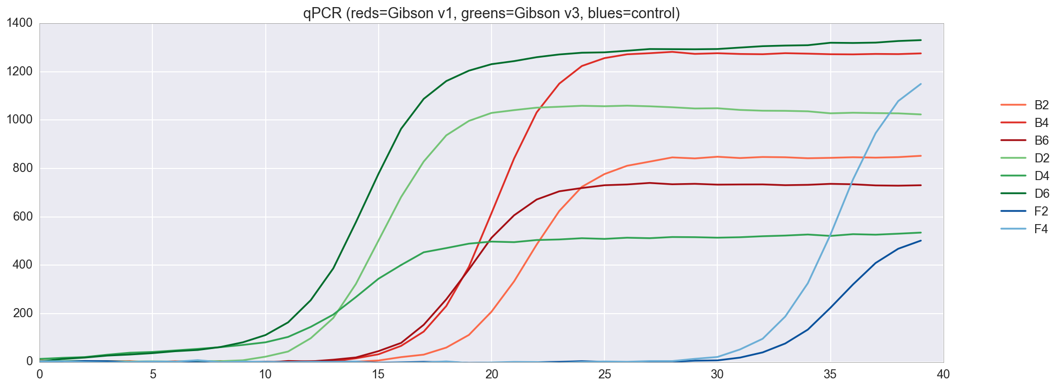
In general, qPCR results look great, with good amplification of both versions of my Gibson assembly and without real amplification in the control group. Since the assembly v3 showed a slightly better result than v1, now we will use it.
The gel is also very clean, showing strong bands just below 1kb in bands B2, B4, B6, D2, D4, D6: this is the size we expect (insertion is about 740bp, and M13 primers are about 40bp up and down). The second lane corresponds to the primers. You can be sure of this, since the F2 and F4 bands contain only primer DNA.

Polyacrylamide gel electrophoresis: c Gibson assembly v3 shows stronger bands (D2, D4, D6), according to the qPCR data above
Transformation is the process of changing the body by adding DNA. In this experiment, we transform E. coli using the sfGFP-expressing plasmid pUC19.
We use the easy-to-use Zymo DH5α Mix & Go strain and the recommended protocol . This strain is part of the standard Transcriptic inventory. In general, transformations can be complex because competent cells are rather fragile, so the simpler and more reliable the protocol, the better. In ordinary molecular biology laboratories, these competent cells would probably be too expensive for general use.
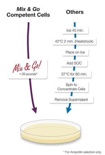
Zymo Mix & Go Cells with Simple Protocol
This protocol is a good example of how difficult it is to adapt human protocols for use by robots and how it can fail unexpectedly. Protocols are sometimes surprisingly vague (“swing the tube from side to side”) based on the general context of molecular biologists, or they may suddenly request advanced image processing (“make sure the pellet is mixed”). People do not mind such tasks, but robots need clearer instructions.
This transformation showed interesting timing issues. The transformation protocol advises that the cells should not remain at room temperature for more than a few seconds and the plate with tubes should be preheated to 37 ° C. Theoretically, you would like to start preheating so that it ends simultaneously with the transformation, but it is unclear how the Transcriptic robots will cope with this situation - as far as I know, there is no way to precisely synchronize the protocol steps. Lack of precise control over time seems to be a common problem with robotic protocols due to the relative inflexibility of the robotic arm, scheduling conflicts, etc. We will have to adjust the protocols accordingly.
Usually there are reasonable solutions: sometimes you just need to use different reagents (for example, more hardy cells, such as Mix & Go above); sometimes you just mortgage actions with a margin (for example, shake ten times instead of three); sometimes you need to come up with special tricks for robots (for example, use a PCR machine for heat stroke).
Of course, the big advantage is that once the protocol has worked once, you can generally rely on it again and again. You can even quantify how reliable the protocol is and improve it over time!
Before starting the transformation with the fully assembled plasmid, I conduct a simple experiment to make sure that the transformation using the usual pUC19 (i.e. without Gibson assembly and without sfGFP DNA insertion) works. pUC19 contains the ampicillin resistance gene, so successful transformation should allow bacteria to grow on plates containing this antibiotic.
I transfer the bacteria directly to the tablet (“6-flat” in Transcriptic terminology), where there is either ampicillin or not. I expect that the transformed bacteria contain the ampicillin resistance gene and therefore will grow. Non-transformed bacteria should not grow.
In the following photographs, we see that without an antibiotic (plate on the left), growth is observed on all six plates, although to a varying degree, which causes concern. It seems that Transcriptic robots do not really cope with uniform distribution, which requires some dexterity.
In the presence of the antibiotic (plate on the right), there is also growth, although again it is inconsistent. The first two plates with antibiotics look strange, with large growth, which is probably the result of adding 55 μl to these plates compared to 10 μl on plates without antibiotics. There are several colonies on the third plate, and in essence this is what I expected to see on all the plates. There should be some growth on the last three plates, but it does not happen. My only explanation for these strange results is that I did not mix the cells and the medium enough, so almost all the cells got into the first two plates.
(I still had to make a positive control on ampicillin with an unchanged bacterium, but I already did this in a previous experiment, so I know that stock ampicillin should kill this strainE. coli . Growth is much weaker on ampicillin plates, although there are much more bacteria there, as expected).
Overall, the transformation worked well enough to continue, although there are some flaws.
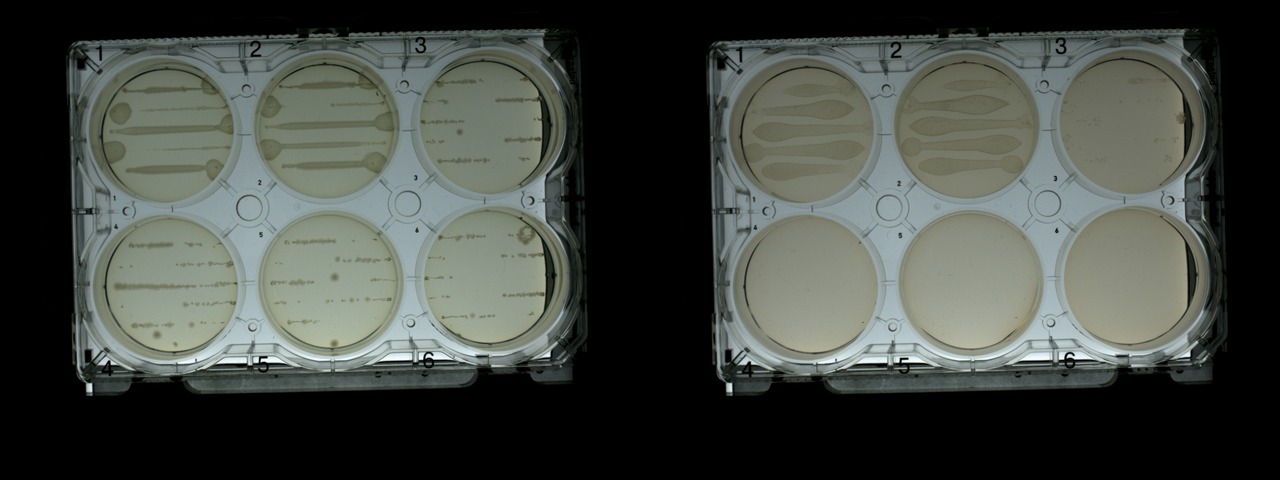
Plates of cells transformed with pUC19 after 18 hours: without antibiotic (left) and with antibiotic (right)
Since the Gibson assembly and simple pUC19 transformation seem to work, you can now try the transformation with a fully assembled plasmid expressing sfGFP.
In addition to the collected insertion, I will also add a little IPTG and X-gal to the plates to see the successful conversion using the blue and white selection method . This additional information is useful, because if the transformation takes place with the usual pUC19, which does not contain sfGFP, it will still give antibiotic resistance.
According to this table , sfGFP glows best at excitation wavelengths of 485 nm / 510 nm. I found that in Transcriptic, 485/535 works better. I guess because 485 and 510 are too similar. I measure bacterial growth at 600 nm ( OD600 ).

Variety of GFP ( biotek )
My IPTG is at a concentration of 1M and should be diluted 1: 1000. In turn, X-gal at a concentration of 20 mg / ml should also be diluted 1: 1000 (20 mg / μl). Therefore, at 2000µl LB I add 2 µl each.
According to one protocol, you must first take 40 μl of X-gal at a concentration of 20 mg / ml and 40 μl of IPTG concentration of 0.1 mM (or 4 μl of IPTG per 1M), and incubate for 30 minutes. This procedure did not work for me, so I just mixed IPTG, X-gal and the corresponding cells and used this mixture directly.
When colonies grow on an ampicillin plate, I can “collect” individual colonies and plant them on a 96-tube plate. For this, there is a special command ( autopick ) in the auto- protocol .
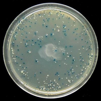
The blue-white screen perfectly showed, mainly, white colonies on plates with antibiotic (1-4) and only blue on plates without antibiotic (5-6). This is exactly what I expected, and I was glad to see it, especially since I used my own IPTG and X-gal, which I sent to Transcriptic.
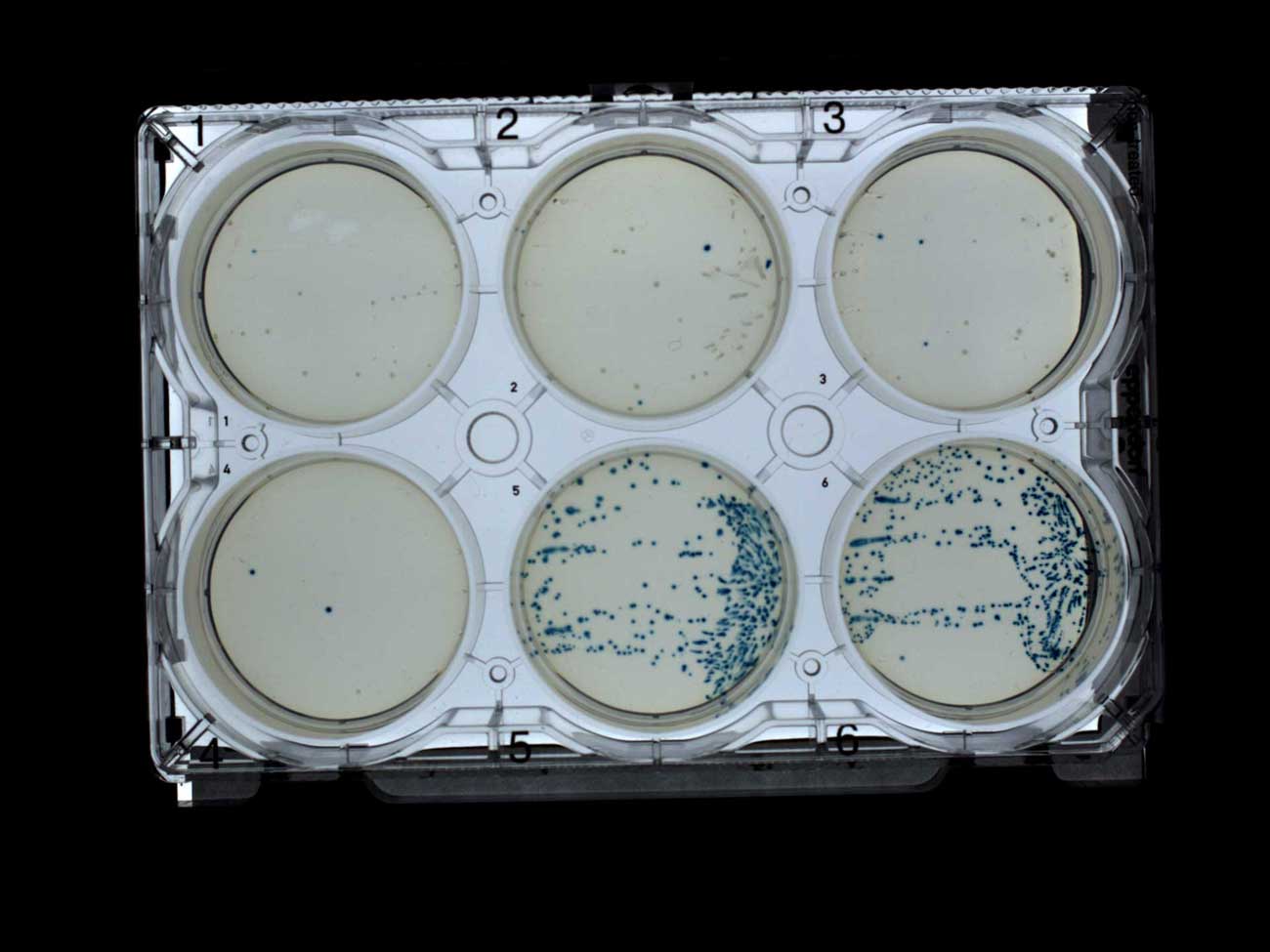
Screening by white-blue selection of plates with ampicillin (1-4) and without antibiotic (5-6)
However, the colony-collecting robot did not work well with these white-blue colonies. The image below was created by subtracting successive photos of the plates after each round of plate selection and increasing the contrast of the differences (in GraphicsMagick ). In this way, I can visualize which colonies were collected (although not ideally, since the collected colonies are not completely removed).
I also signed the image with the number of colonies collected by the Transcriptic robot. It was assumed that he would collect a maximum of 10 colonies from the first five plates. However, in general, several colonies were collected, and these are usually blue colonies. The robot only managed to find ten colonies on a control plate with only blue colonies. My working theory is that a colony collecting robot preferably collects blue colonies because they are more contrasting.
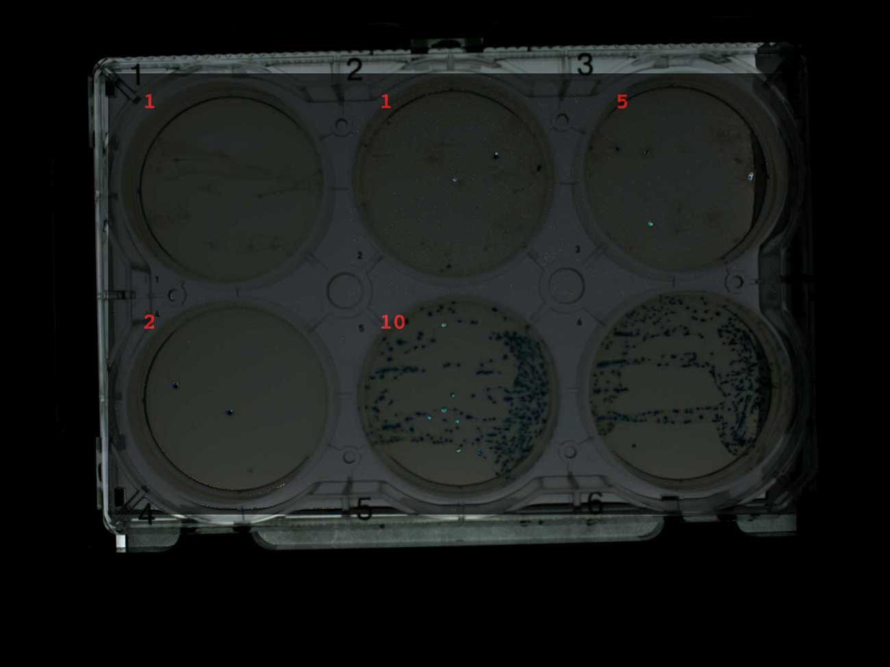
Screening plates for blue-white selection with ampicillin (1-4) and without antibiotic (5-6), indicating the number of collected colonies
Blue and white screening served a specific purpose. He showed that most colonies transform correctly. At least there is an insertion. However, for better colony collection, I repeated the experiment without X-gal.
Only with white colonies did the robot collector successfully assemble ten colonies from each of the first five plates. It can be assumed that in most of the collected colonies there are successful insertions.
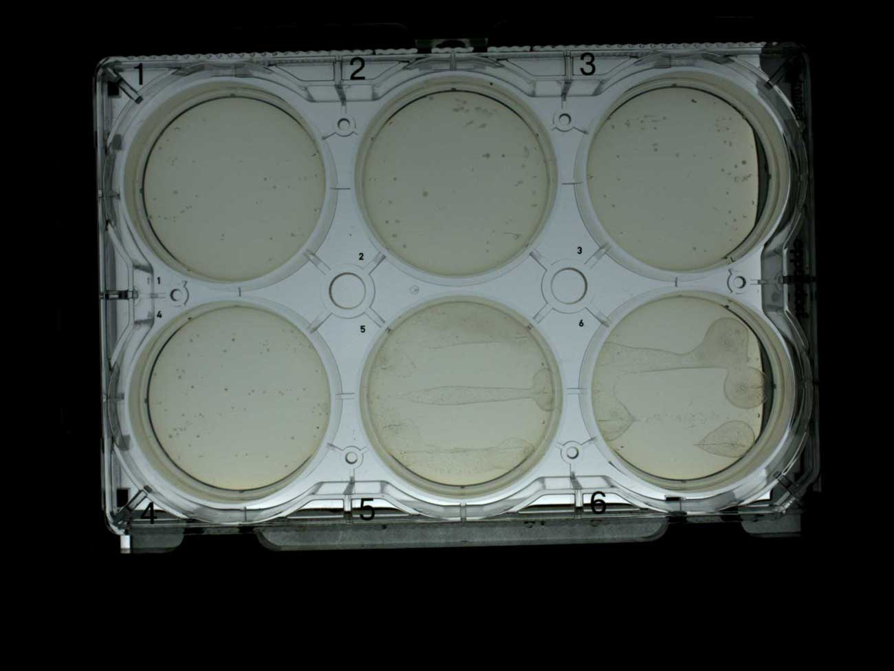
Colonies growing on plates with ampicillin (1-4) and without antibiotic (5-6)
After growing 50 selected colonies on a 96-tube plate for 20 hours, I measure fluorescence to check the expression of sfGFP. Transcriptic uses a Tecan Infinite reader to measure fluorescence and absorption (and luminescence, if you like) .
In theory, in any colony, a plasmid must be assembled with growth, since it needs antibiotic resistance to grow, and each plasmid collected expresses sfGFP. There are actually many reasons why this may not be the case, not least because you can lose the sfGFP gene from the plasmid without losing ampicillin resistance. A bacterium that loses the sfGFP gene has an advantage in selection over its competitors, because it does not spend extra energy, and taking into account a sufficient number of generations of growth, this will certainly happen.
I collect absorption data (OD600) and fluorescence every four hours for 20 hours (about 60 generations).
We place on the chart the data of the 20th hour and traces of previous measurements. In fact, I am only interested in the latest data, since it is then that a fluorescence peak should be observed.
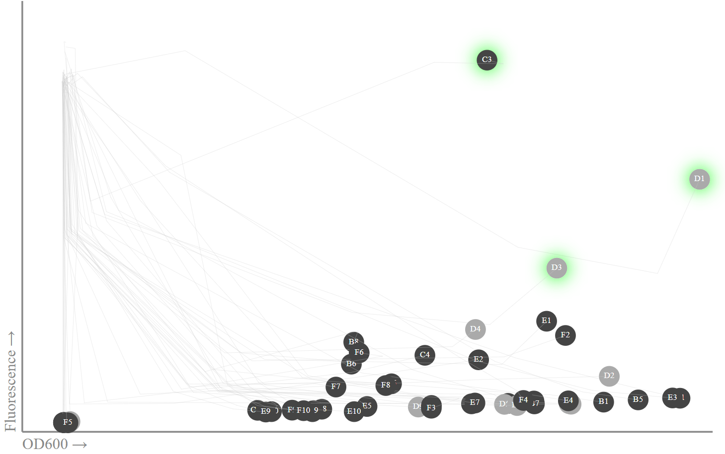
Fluorescence and OD600: colonies with ampicillin are black, control colonies without ampicillin are gray. The colonies were highlighted in green, where I confirmed the sfGFP protein sequence was correct.
Run miniprep to extract plasmid DNA, then Sanger sequencing using M13 primers. Unfortunately, for some reason, miniprep is currently only available through the Transcriptic web protocol, and not through auto-protocol. I will sequence the three tubes with the highest fluorescence readings (C1, D1, D3) and the other three (B1, B3, E1), aligning the sequences with sfGFP using muscle .
In tubes C1, D3, and D3, the perfect match for my original sfGFP sequence, while in B1, B3, and E1, coarse mutations or alignment simply fails.
The results are good, although some aspects are surprising. For example, a fluorescence reader, for no apparent reason, starts at time 0 with very high values (40,000 blocks). By the 20th hour, he had calmed down to a more reasonable pattern with a clear correlation between OD600 and fluorescence (I suppose due to a small overlap in the spectra), plus some emissions with high fluorescence. Surprisingly, it can be one, three or, possibly, 11-15 emissions.
Some of the tubes with high fluorescence values are located in control tubes (i.e., without ampicillin, they are colored gray), which is surprising since there is no selection pressure in these tubes, therefore, plasmid loss can be expected).
Based on fluorescence data and sequencing results, it appears that only three of the 50 colonies produce sfGFP and fluoresce. This is not as much as I expected. However, since there have been three separate growth stages (on the plate, in vitro, for miniprep), about 200 generations of growth have undergone to this stage of the cell, so there were quite a lot of opportunities for mutations to occur.
There should be ways to make the process more efficient, especially since I am far from an expert on these protocols. However, we successfully produced transformed cells with expression of the engineered GFP using only the Python code!
Depending on how to measure, the cost of this experiment was about $ 360, not including the money for debugging:
I think that the cost can be reduced to $ 250-300 with some improvements. For example, robotic collection of 50 colonies is suspiciously expensive and probably can be abandoned.
In my experience, this price seems high for some (molecular biologists) and low for others (IT people). Since Transcriptic basically just charges the price list reagents, the main difference in costs is labor. The robot is already quite cheap at an hour, and he would not mind getting up in the middle of the night to photograph a plate. Once the protocols are approved, it is hard to imagine that even a graduate student would be cheaper, especially considering the opportunity costs.
For clarity, I am only talking about replacing routine protocols. Of course, the development of advanced protocols will continue to be carried out by qualified molecular biologists, but many exciting areas of science use boring routine protocols. Until recently, many laboratories produced their own oligonucleotides, but now few people worry about this: it just does not cost anyone any time, not even graduate students, when the IDT sends them to you within a few days.
Obviously, I really believe in the future of robotic laboratories. There are some really funny and useful things in experimenting with robots, especially if you are primarily involved in computing and are allergic to latex gloves and manual labor:
Of course, there are some drawbacks, especially since the tools have just begun to develop. If we compare with the Internet, then we are in the 1994 area:
Although there is a lot of code and quite a lot of debugging, I think it’s possible to create some kind of software that takes a sequence of proteins as input and creates bacteria with the expression of this protein at the output.
For this to work, several things must happen:
In many applications, you also want to purify your protein (via a column ), or perhaps just make the bacteria secrete it. Suppose that we can soon do this in a cloud lab, or that we can conduct in vivo experiments (i.e., inside a bacterial cell).
There are many possibilities for the protocol to actually work better than humans, for example: the design of promoters and RBS to optimize expression specific to your sequence; statistics of the probability of success of an experiment based on comparable experiments; automated gel analysis.
After all this, it may not be completely clear why to create such a protein. Here are some ideas:
For new ideas on what is possible with protein design, look at hundreds of iGEM projects .
In the end, I want to thank Transcriptic Ben Miles for his help in completing this project.
Surprisingly, we are very close to creating any protein we want without leaving the Jupyter notebook thanks to the latest developments in genomics, synthetic biology, and more recently - in cloud labs.
In this article, I will show Python code from the idea of a protein to its expression in a bacterial cell, without touching a pipette or talking to anyone. The total cost will be only a few hundred dollars! Using the terminology of Vijaya Pande from A16Z , this is Biology 2.0.
More specifically, in the article, the Python code of the cloud lab does the following:
- Synthesis of a DNA sequence that encodes any protein that I want.
- Cloning this synthetic DNA into a vector that can express it.
- Transformation of bacteria with this vector and confirmation that expression is occurring.
Python setup
First, the general Python settings that are needed for any Jupyter notepad. We import some useful Python modules and create some utility functions, mainly for data visualization.
The code
import re
import json
import logging
import requests
import itertools
import numpy as np
import seaborn as sns
import pandas as pd
import matplotlib as mpl
import matplotlib.pyplot as plt
from io import StringIO
from pprint import pprint
from Bio.Seq import Seq
from Bio.Alphabet import generic_dna
from IPython.display import display, Image, HTML, SVG
def uprint(astr): print(astr + "\n" + "-"*len(astr))
def show_html(astr): return display(HTML('{}'.format(astr)))
def show_svg(astr, w=1000, h=1000):
SVG_HEAD = ''''''
SVG_START = ''''))
def table_print(rows, header=True):
html = [""]
html_row = "".format('bold' if header is True else 'normal', html_row))
for row in rows[1:]:
html_row = "".format(html_row))
html.append("".join(k for k in rows[0])
html.append(" {} ".join(row)
html.append(" {:}
")
show_html(''.join(html))
def clean_seq(dna):
dna = re.sub("\s","",dna)
assert all(nt in "ACGTN" for nt in dna)
return Seq(dna, generic_dna)
def clean_aas(aas):
aas = re.sub("\s","",aas)
assert all(aa in "ACDEFGHIKLMNPQRSTVWY*" for aa in aas)
return aas
def Images(images, header=None, width="100%"): # to match Image syntax
if type(width)==type(1): width = "{}px".format(width)
html = ["".format(width)]
if header is not None:
html += ["".format(h) for h in header] + [""]
for image in images:
html.append("".format(image))
html.append("{} 
")
show_html(''.join(html))
def new_section(title, color="#66aa33", padding="120px"):
style = "text-align:center;background:{};padding:{} 10px {} 10px;".format(color,padding,padding)
style += "color:#ffffff;font-size:2.55em;line-height:1.2em;"
return HTML('{}'.format(style, title))
# Show or hide text
HTML("""
""")
# Plotting style
plt.rc("axes", titlesize=20, labelsize=15, linewidth=.25, edgecolor='#444444')
sns.set_context("notebook", font_scale=1.2, rc={})
%matplotlib inline
%config InlineBackend.figure_format = 'retina' # or 'svg'Cloud labs
Like AWS or any computing cloud, the cloud lab has molecular biology equipment, as well as robots that it leases over the Internet. You can issue instructions to your robots by clicking a few buttons on the interface or by writing code that programs them yourself. It is not necessary to write your own protocols, as I will do here, a significant part of molecular biology is standard routine tasks, so it is usually better to rely on a reliable alien protocol that showed good interaction with robots.
Recently, a number of companies with cloud labs have appeared: Transcriptic , Autodesk Wet Lab Accelerator (beta, and built on the basis of Transcriptic), Arcturus BioCloud (beta),Emerald Cloud Lab (beta), Synthego (not yet launched). There are even companies built on top of cloud labs such as Desktop Genetics , which specializes in CRISPR. Scientific articles about the use of cloud labs in real science are starting to appear .
At the time of this writing, only Transcriptic is in the public domain, so we will use it. As I understand it, most of the Transcriptic business is built on automating common protocols, and writing your own protocols in Python (as I will do in this article) is less common.
Transcriptic “working cell” with refrigerators at the bottom and various laboratory equipment at the stand
I will give Transcriptic robots instructions onauto protocol . Autoprotocol is a JSON-based language for writing protocols for laboratory robots (and humans, as it were). Autoprotocol is mainly made on this Python library . The language was originally created and is still supported by Transcriptic, but, as I understand it, it is completely open. There is good documentation .
An interesting idea is that on the auto-protocol you can write instructions for people in remote laboratories - say, in China or India - and potentially get some advantages from using both people (their judgment) and robots (lack of judgment). We need to mention protocols.io here , this is an attempt to standardize protocols to improve reproducibility, but for humans, not robots.
"instructions": [
    {
      "to": [
        {
          "well": "water/0",
          "volume": "500.0:microliter"
        }
      ],
      "op": "provision",
      "resource_id": "rs17gmh5wafm5p"
    },
    ...
]
Autoprotocol fragment example
Python settings for molecular biology
In addition to importing standard libraries, I will need some specific molecular biological utilities. This code is mainly for auto-protocol and Transcriptic.
The concept of “dead volume” is often found in code. This means the last drop of liquid that Transcriptic robots cannot take with a pipette from the tubes (because they cannot see it!). You have to spend a lot of time to make sure that the flasks have enough material.
The code
import autoprotocol
from autoprotocol import Unit
from autoprotocol.container import Container
from autoprotocol.protocol import Protocol
from autoprotocol.protocol import Ref # "Link a ref name (string) to a Container instance."
import requests
import logging
# Transcriptic authorization
org_name = 'hgbrian'
tsc_headers = {k:v for k,v in json.load(open("auth.json")).items() if k in ["X_User_Email","X_User_Token"]}
# Transcriptic-specific dead volumes
_dead_volume = [("96-pcr",3), ("96-flat",25), ("96-flat-uv",25), ("96-deep",15),
                ("384-pcr",2), ("384-flat",5), ("384-echo",15),
                ("micro-1.5",15), ("micro-2.0",15)]
dead_volume = {k:Unit(v,"microliter") for k,v in _dead_volume}
def init_inventory_well(well, headers=tsc_headers, org_name=org_name):
    """Initialize well (set volume etc) for Transcriptic"""
    def _container_url(container_id):
        return 'https://secure.transcriptic.com/{}/samples/{}.json'.format(org_name, container_id)
    response = requests.get(_container_url(well.container.id), headers=headers)
    response.raise_for_status()
    container = response.json()
    well_data = container['aliquots'][well.index]
    well.name = "{}/{}".format(container["label"], well_data['name']) if well_data['name'] is not None else container["label"]
    well.properties = well_data['properties']
    well.volume = Unit(well_data['volume_ul'], 'microliter')
    if 'ERROR' in well.properties:
        raise ValueError("Well {} has ERROR property: {}".format(well, well.properties["ERROR"]))
    if well.volume < Unit(20, "microliter"):
        logging.warn("Low volume for well {} : {}".format(well.name, well.volume))
    return True
def touchdown(fromC, toC, durations, stepsize=2, meltC=98, extC=72):
    """Touchdown PCR protocol generator"""
    assert 0 < stepsize < toC < fromC
    def td(temp, dur): return {"temperature":"{:2g}:celsius".format(temp), "duration":"{:d}:second".format(dur)}
    return [{"cycles": 1, "steps": [td(meltC, durations[0]), td(C, durations[1]), td(extC, durations[2])]}
            for C in np.arange(fromC, toC-stepsize, -stepsize)]
def convert_ug_to_pmol(ug_dsDNA, num_nts):
    """Convert ug dsDNA to pmol"""
    return float(ug_dsDNA)/num_nts * (1e6 / 660.0)
def expid(val):
    """Generate a unique ID per experiment"""
    return "{}_{}".format(experiment_name, val)
def µl(microliters):
    """Unicode function name for creating microliter volumes"""
    return Unit(microliters,"microliter")
DNA synthesis and synthetic biology
Despite its connection with modern synthetic biology, DNA synthesis is a fairly old technology. For decades, we have been able to make oligonucleotides (that is, DNA sequences up to 200 bases). However, it was always expensive, and chemistry never allowed long DNA sequences. Recently, it has become possible at a reasonable price to synthesize whole genes (up to thousands of bases). This achievement truly opens the era of “synthetic biology”.
The company Synthetic Genomics Craig Venter's synthetic biology has advanced furthest, synthesizing the whole organism - more than a million bases in length. As the length of the DNA increases, the problem is no longer synthesis, but assembly (i.e., stitching together synthesized DNA sequences). With each assembly, you can double the DNA length (or more), so after a dozen or so iterations, you get a rather long molecule ! The distinction between synthesis and assembly should soon become clear to the end user.
Moore's Law?
The price of DNA synthesis is falling pretty fast, from over $ 0.30 a year ago two to about $ 0.10 today, but it is developing more like bacteria than processors. In contrast, DNA sequencing prices are falling faster than Moore’s law. A target of $ 0.02 per base is set as an inflection point where you can replace a lot of time-consuming DNA manipulations with simple synthesis. For example, at this price, you can synthesize a whole 3kb plasmid for $ 60 and skip a bunch of molecular biology. I hope we will achieve this in a couple of years.
DNA synthesis prices compared to DNA sequencing prices, price for 1 base (Carlson, 2014)
DNA synthesis companies
There are several large companies in the field of DNA synthesis: IDT is the largest producer of oligonucleotides, and can also produce longer (up to 2kb) “gene fragments” ( gBlocks ). Gen9 , Twist, and DNA 2.0 typically specialize in longer DNA sequences - these are gene synthesis companies. There are also some interesting new companies, such as Cambrian Genomics and Genesis DNA , that are working on next-generation synthesis methods.
Other companies such as Amyris , Zymergen and Ginkgo Bioworks, use the DNA synthesized by these companies to work at the body level. Synthetic Genomics does this too, but it synthesizes DNA itself.
Ginkgo recently struck a deal with Twist to make 100 million bases: the largest deal I've seen. This proves that we live in the future, Twist even advertised a promotional code on Twitter: when you buy 10 million DNA bases (almost the entire yeast genome!), You get another 10 million for free.
Twitter Twist Niche Offer
Part One: Experiment Design
Green fluorescent protein
In this experiment, we synthesize a DNA sequence for a simple, green fluorescent protein (GFP). The GFP protein was first found in a jellyfish that fluoresces under ultraviolet light. This is an extremely useful protein because it is easy to detect its expression simply by measuring fluorescence. There are GFP options that produce yellow, red, orange, and other colors.
It is interesting to see how various mutations affect the color of a protein, and this is a potentially interesting machine learning problem. More recently, you would have to spend a lot of time in the laboratory for this, but now I will show you that it is (almost) as easy as editing a text file!
Technically, my GFP is a Super Folder Option (sfGFP) with some mutations to improve quality.
In superfolder-GFP (sfGFP), some mutations give it certain useful properties.
GFP structure (visualized using PV )
GFP synthesis in Twist
I was fortunate enough to get into Twist's alpha testing program, so I used their DNA synthesis service (they kindly placed my tiny order - thanks, Twist!). This is a new company in our field, with a new simplified synthesis process. Their prices are around $ 0.10 per base or lower , but they are still in beta , and the alpha program in which I participated was closed. Twist raised about $ 150 million, so their technology is lively.
I sent my DNA sequence to Twist as an Excel spreadsheet (there is no API yet, but I guess it will be soon), and they sent the synthesized DNA directly to my box in the Transcriptic laboratory (I also used IDT for synthesis, but they did not send DNA right in Transcriptic, which spoils the fun a bit).
Obviously, this process has not yet become a typical use case and requires some support, but it worked, so that the entire pipeline remains virtual. Without this, I probably would need access to the laboratory - many companies will not send DNA or reagents to their home address.
GFP is harmless, so any kind is highlighted
Plasmid vector
To express this protein in bacteria, the gene needs to live somewhere, otherwise the synthetic DNA encoding the gene simply degrades instantly. As a rule, in molecular biology we use a plasmid, a piece of round DNA that lives outside the bacterial genome and expresses proteins. Plasmids are a convenient way for bacteria to share useful, stand-alone functional modules, such as antibiotic resistance. There can be hundreds of plasmids in a cell.
Widely used terminology is that a plasmid is a vector , and synthetic DNA is an insertion (insertion). So, here we are trying to clone the insertion into a vector, and then transform the bacteria using the vector.
Bacterial genome and plasmid (not to scale!) ( Wikipedia )
pUC19
I chose a fairly standard plasmid in the pUC19 series . This plasmid is very often used, and since it is available as part of the standard Transcriptic inventory, we do not need to send anything to them.
Structure of pUC19: the main components are the gene for resistance to ampicillin, lacZα, MCS / polylinker and the origin of replication (Wikipedia)
pUC19 has a nice function: since it contains the lacZα gene, you can use the blue-white selection method and see which colonies are successfully The insertion has passed. Two chemicals are needed: IPTG and X-gal , and the circuit works as follows:
- IPTG induces lacZα expression.
- If lacZα is deactivated via DNA inserted at the multiple cloning site ( MCS / polylinker ) in lacZα, then the plasmid cannot hydrolyze X-gal and these colonies will be white instead of blue.
- Therefore, a successful insertion produces white colonies, and a failed insertion produces blue colonies.
Blue-white selection shows where lacZα expression was deactivated ( Wikipedia )
The openwetware documentation says:
E. coli DH5α does not require IPTG to induce expression from the lac promoter, even if a Lac repressor is expressed in the strain. The copy number of most plasmids exceeds the number of repressors in the cells. If you need maximum expression, add IPTG to a final concentration of 1 mM.
Synthetic DNA Sequences
SfGFP DNA sequence
It is easy to obtain the DNA sequence for sfGFP by taking the protein sequence and encoding it with codons suitable for the host organism (here, E. coli ). This is a medium-sized protein with 236 amino acids, so at 10 cents DNA synthesis costs about $ 70 per base .
Wolfram Alpha, calculation of the cost of synthesis
The first 12 bases of our sfGFP are the Shine-Delgarno sequence , which I added myself, which theoretically should increase expression (AGGAGGACAGCT, then ATG ( start codon ) launches the protein). According to a computing tool developed by Salis Lab ( lecture slides), we can expect medium to high expression of our protein (translation initiation rate of 10,000 “arbitrary units”).
sfGFP_plus_SD = clean_seq("""
AGGAGGACAGCTATGTCGAAAGGAGAAGAACTGTTTACCGGTGTGGTTCCGATTCTGGTAGAACTGGA
TGGGGACGTGAACGGCCATAAATTTAGCGTCCGTGGTGAGGGTGAAGGGGATGCCACAAATGGCAAAC
TTACCCTTAAATTCATTTGCACTACCGGCAAGCTGCCGGTCCCTTGGCCGACCTTGGTCACCACACTG
ACGTACGGGGTTCAGTGTTTTTCGCGTTATCCAGATCACATGAAACGCCATGACTTCTTCAAAAGCGC
CATGCCCGAGGGCTATGTGCAGGAACGTACGATTAGCTTTAAAGATGACGGGACCTACAAAACCCGGG
CAGAAGTGAAATTCGAGGGTGATACCCTGGTTAATCGCATTGAACTGAAGGGTATTGATTTCAAGGAA
GATGGTAACATTCTCGGTCACAAATTAGAATACAACTTTAACAGTCATAACGTTTATATCACCGCCGA
CAAACAGAAAAACGGTATCAAGGCGAATTTCAAAATCCGGCACAACGTGGAGGACGGGAGTGTACAAC
TGGCCGACCATTACCAGCAGAACACACCGATCGGCGACGGCCCGGTGCTGCTCCCGGATAATCACTAT
TTAAGCACCCAGTCAGTGCTGAGCAAAGATCCGAACGAAAAACGTGACCATATGGTGCTGCTGGAGTT
CGTGACCGCCGCGGGCATTACCCATGGAATGGATGAACTGTATAAA""")
print("Read in sfGFP plus Shine-Dalgarno: {} bases long".format(len(sfGFP_plus_SD)))
sfGFP_aas = clean_aas("""MSKGEELFTGVVPILVELDGDVNGHKFSVRGEGEGDATNGKLTLKFICTTGKLPVPWPTLVTTLTYG
VQCFSRYPDHMKRHDFFKSAMPEGYVQERTISFKDDGTYKTRAEVKFEGDTLVNRIELKGIDFKEDGNILGHKLEYNFNSHNVYITADKQKN
GIKANFKIRHNVEDGSVQLADHYQQNTPIGDGPVLLPDNHYLSTQSVLSKDPNEKRDHMVLLEFVTAAGITHGMDELYK""")
assert sfGFP_plus_SD[12:].translate() == sfGFP_aas
print("Translation matches protein with accession 532528641")
Read in sfGFP plus Shine-Dalgarno: 726 bases long Translation matches protein with accession 532528641
PUC19 DNA sequence
First, I check that the pUC19 sequence that I downloaded from the NEB has the correct length and it includes the expected polylinker .
pUC19_fasta = !cat puc19fsa.txt
pUC19_fwd = clean_seq(''.join(pUC19_fasta[1:]))
pUC19_rev = pUC19_fwd.reverse_complement()
assert all(nt in "ACGT" for nt in pUC19_fwd)
assert len(pUC19_fwd) == 2686
pUC19_MCS = clean_seq("GAATTCGAGCTCGGTACCCGGGGATCCTCTAGAGTCGACCTGCAGGCATGCAAGCTT")
print("Read in pUC19: {} bases long".format(len(pUC19_fwd)))
assert pUC19_MCS in pUC19_fwd
print("Found MCS/polylinker")
Read in pUC19: 2686 bases long Found MCS / polylinker
We do some basic QCs to make sure that EcoRI and BamHI are present in pUC19 only once (the following restriction enzymes are available in the default Transcriptic inventory: PstI , PvuII , EcoRI , BamHI , BbsI , BsmBI ).
REs = {"EcoRI":"GAATTC", "BamHI":"GGATTC"}
for rename, res in REs.items():
    assert (pUC19_fwd.find(res) == pUC19_fwd.rfind(res) and
            pUC19_rev.find(res) == pUC19_rev.rfind(res))
    assert (pUC19_fwd.find(res) == -1 or pUC19_rev.find(res) == -1 or
            pUC19_fwd.find(res) == len(pUC19_fwd) - pUC19_rev.find(res) - len(res))
print("Asserted restriction enzyme sites present only once: {}".format(REs.keys()))
Now we look at the lacZα sequence and verify that there is nothing unexpected. For example, it should begin with Met and end with a stop codon. It is also easy to confirm that this is the full 324bp lacZα ORF by loading the pUC19 sequence into the free snapgene viewer .
lacZ = pUC19_rev[2217:2541]
print("lacZα sequence:\t{}".format(lacZ))
print("r_MCS sequence:\t{}".format(pUC19_MCS.reverse_complement()))
lacZ_p = lacZ.translate()
assert lacZ_p[0] == "M" and not "*" in lacZ_p[:-1] and lacZ_p[-1] == "*"
assert pUC19_MCS.reverse_complement() in lacZ
assert pUC19_MCS.reverse_complement() == pUC19_rev[2234:2291]
print("Found MCS once in lacZ sequence")
lacZ sequence: ATGACCATGATTACGCCAAGCTTGCATGCCTGCAGGTCGACTCTAGAGGATCCCCGGGTACCGAGCTCGAATTCACTGGCCGTCGTTTTACAACGTCGTGACTGGGAAAACCCTGGCGTTACCCAACTTAATCGCCTTGCAGCACATCCCCCTTTCGCCAGCTGGCGTAATAGCGAAGAGGCCCGCACCGATCGCCCTTCCCAACAGTTGCGCAGCCTGAATGGCGAATGGCGCCTGATGCGGTATTTTCTCCTTACGCATCTGTGCGGTATTTCACACCGCATATGGTGCACTCTCAGTACAATCTGCTCTGATGCCGCATAG r_MCS sequence: AAGCTTGCATGCCTGCAGGTCGACTCTAGAGGATCCCCGGGTACCGAGCTCGAATTC Found MCS once in lacZ sequence
Сборка методом Гибсона
Assembling DNA simply means crosslinking fragments. Usually you collect several DNA fragments into a longer segment, and then clone it into a plasmid or genome. In this experiment, I want to clone one segment of DNA into the pUC19 plasmid below the lac promoter for expression in E. coli .
There are many cloning methods (e.g. NEB , openwetware , addgene ). Here I will use the Gibson assembly ( developed by Daniel Gibsonat Synthetic Genomics in 2009), which is not necessarily the cheapest method, but simple and flexible. You just need to put the DNA that you want to collect (with the appropriate overlap) in a test tube with the Gibson Assembly Master Mix, and it will assemble itself!
Gibson Assembly Review ( NEB )
Raw material
We start with 100 ng of synthetic DNA in 10 μl of liquid. This equals 0.21 picomoles of DNA or a concentration of 10 ng / μl.
pmol_sfgfp = convert_ug_to_pmol(0.1, len(sfGFP_plus_SD))
print("Insert: 100ng of DNA of length {:4d} equals {:.2f} pmol".format(len(sfGFP_plus_SD), pmol_sfgfp))
Insert: 100ng of DNA of length 726 equals 0.21 pmol
According to the NEB assembly protocol , this is enough source material:
NEB рекомендует в общей сложности 0,02-0,5 пикомолей фрагментов ДНК, когда в вектор собирается 1 или 2 фрагмента, или 0,2-1,0 пикомолей фрагментов ДНК, когда собираются 4-6 фрагментов.
0.02-0.5 пмолей * X мкл
* Оптимизированная эффективность клонирования составляет 50-100 нг векторов с 2-3-кратным избытком инсерций. Используйте в 5 раз больше инсерций, если размер меньше 200 bps. Общий объём нефильтрованных фрагментов PCR в реакции сборки Гибсона не должен превышать 20%.
NEBuilder для сборки Гибсона
NEBuilder from the company Biolab - it really is a great tool for creating a protocol Gibson assembly. It even generates you a comprehensive four-page PDF with all the information. Using this tool, we develop a protocol for cutting pUC19 with EcoRI, and then use PCR [PCR, polymerase chain reaction allows to achieve a significant increase in small concentrations of certain DNA fragments in biological material - approx. per.] to add fragments of the appropriate size to the insertion.
Part two: experiment
The experiment consists of four stages:
- Polymerase chain insertion reaction to add material with a flanking sequence.
- Cutting a plasmid to accommodate insertion.
- Assembly by Gibson insertion and plasmids.
- Transformation of bacteria using the assembled plasmid.
Step 1. PCR insertion
Gibson assembly depends on the DNA sequence that you collect, having some overlapping sequence (see NEB protocol with detailed instructions above). In addition to simple amplification, PCR also allows you to add a flanking DNA sequence by simply including an additional sequence in the primers (can also be cloned using only OE-PCR ).
We synthesize primers according to the NEB protocol above. I tried the Quickstart protocol on the Transcriptic site, but there is still an auto- protocol command. Transcriptic itself does not synthesize oligonucleotides, so after 1-2 days of waiting, these primers magically appear in my inventory (note that the gene-specific part of the primers is indicated in upper case below, but these are just cosmetic things).
insert_primers = ["aaacgacggccagtgTTTATACAGTTCATCCATTCCATG", "cgggtaccgagctcgAGGAGGACAGCTATGTCG"]Primer Analysis
You can analyze the properties of these primers using the IDT OligoAnalyzer . when debugging a PCR experiment, it is useful to know the melting points and the likelihood of a side effect of primer dimer , although the NEB protocol will almost certainly select primers with good properties.
Gene-specific portion of flank (uppercase)
  Melt temperature: 51C, 53.5C
Full sequence
  Melt temperature: 64.5C, 68.5C
  Hairpin: -.4dG, -5dG
  Self-dimer: -9dG, -16dG
  Heterodimer: -6dG
I went through many iterations of PCR before getting satisfactory results, including experiments with several different brands of PCR blends. Since each of these iterations can take several days (depending on the length of the queue to the laboratory), it is worth spending time on debugging in advance: this saves a lot of time in the long run. As the power of the cloud lab increases, this problem should become less acute. However, it is unlikely that your first protocol will succeed - there are too many variables.
The code
""" PCR overlap extension of sfGFP according to NEB protocol.
v5: Use 3/10ths as much primer as the v4 protocol.
v6: more complex touchdown pcr procedure. The Q5 temperature was probably too hot
v7: more time at low temperature to allow gene-specific part to anneal
v8: correct dNTP concentration, real touchdown
"""
p = Protocol()
# ---------------------------------------------------
# Set up experiment
#
experiment_name = "sfgfp_pcroe_v8"
template_length = 740
_options = {'dilute_primers' : False, # if working stock has not been made
            'dilute_template': False, # if working stock has not been made
            'dilute_dNTP'    : False, # if working stock has not been made
            'run_gel'        : True,  # run a gel to see the plasmid size
            'run_absorbance' : False, # check absorbance at 260/280/320
            'run_sanger'     : False} # sanger sequence the new sequence
options = {k for k,v in _options.items() if v is True}
# ---------------------------------------------------
# Inventory and provisioning
# https://developers.transcriptic.com/v1.0/docs/containers
#
# 'sfgfp2':              'ct17yx8h77tkme', # inventory; sfGFP tube #2, micro-1.5, cold_20
# 'sfgfp_puc19_primer1': 'ct17z9542mrcfv', # inventory; micro-2.0, cold_4
# 'sfgfp_puc19_primer2': 'ct17z9542m5ntb', # inventory; micro-2.0, cold_4
# 'sfgfp_idt_1ngul':     'ct184nnd3rbxfr', # inventory; micro-1.5, cold_4, (ERROR: no template)
#
inv = {
    'Q5 Polymerase':                     'rs16pcce8rdytv', # catalog; Q5 High-Fidelity DNA Polymerase
    'Q5 Buffer':                         'rs16pcce8rmke3', # catalog; Q5 Reaction Buffer
    'dNTP Mixture':                      'rs16pcb542c5rd', # catalog; dNTP Mixture (25mM?)
    'water':                             'rs17gmh5wafm5p', # catalog; Autoclaved MilliQ H2O
    'sfgfp_pcroe_v5_puc19_primer1_10uM': 'ct186cj5cqzjmr', # inventory; micro-1.5, cold_4
    'sfgfp_pcroe_v5_puc19_primer2_10uM': 'ct186cj5cq536x', # inventory; micro-1.5, cold_4
    'sfgfp1':                            'ct17yx8h759dk4', # inventory; sfGFP tube #1, micro-1.5, cold_20
}
# Existing inventory
template_tube = p.ref("sfgfp1", id=inv['sfgfp1'], cont_type="micro-1.5", storage="cold_4").well(0)
dilute_primer_tubes = [p.ref('sfgfp_pcroe_v5_puc19_primer1_10uM', id=inv['sfgfp_pcroe_v5_puc19_primer1_10uM'], cont_type="micro-1.5", storage="cold_4").well(0),
                       p.ref('sfgfp_pcroe_v5_puc19_primer2_10uM', id=inv['sfgfp_pcroe_v5_puc19_primer2_10uM'], cont_type="micro-1.5", storage="cold_4").well(0)]
# New inventory resulting from this experiment
dilute_template_tube = p.ref("sfgfp1_0.25ngul",  cont_type="micro-1.5", storage="cold_4").well(0)
dNTP_10uM_tube       = p.ref("dNTP_10uM",        cont_type="micro-1.5", storage="cold_4").well(0)
sfgfp_pcroe_out_tube = p.ref(expid("amplified"), cont_type="micro-1.5", storage="cold_4").well(0)
# Temporary tubes for use, then discarded
mastermix_tube = p.ref("mastermix", cont_type="micro-1.5", storage="cold_4",  discard=True).well(0)
water_tube =     p.ref("water",     cont_type="micro-1.5", storage="ambient", discard=True).well(0)
pcr_plate =      p.ref("pcr_plate", cont_type="96-pcr",    storage="cold_4",  discard=True)
if 'run_absorbance' in options:
    abs_plate = p.ref("abs_plate", cont_type="96-flat", storage="cold_4", discard=True)
# Initialize all existing inventory
all_inventory_wells = [template_tube] + dilute_primer_tubes
for well in all_inventory_wells:
    init_inventory_well(well)
    print(well.name, well.volume, well.properties)
# -----------------------------------------------------
# Provision water once, for general use
#
p.provision(inv["water"], water_tube, µl(500))
# -----------------------------------------------------
# Dilute primers 1/10 (100uM->10uM) and keep at 4C
#
if 'dilute_primers' in options:
    for primer_num in (0,1):
        p.transfer(water_tube, dilute_primer_tubes[primer_num], µl(90))
        p.transfer(primer_tubes[primer_num], dilute_primer_tubes[primer_num], µl(10), mix_before=True, mix_vol=µl(50))
        p.mix(dilute_primer_tubes[primer_num], volume=µl(50), repetitions=10)
# -----------------------------------------------------
# Dilute template 1/10 (10ng/ul->1ng/ul) and keep at 4C
# OR
# Dilute template 1/40 (10ng/ul->0.25ng/ul) and keep at 4C
#
if 'dilute_template' in options:
    p.transfer(water_tube, dilute_template_tube, µl(195))
    p.mix(dilute_template_tube, volume=µl(100), repetitions=10)
# Dilute dNTP to exactly 10uM
if 'dilute_DNTP' in options:
    p.transfer(water_tube,           dNTP_10uM_tube, µl(6))
    p.provision(inv["dNTP Mixture"], dNTP_10uM_tube, µl(4))
# -----------------------------------------------------
# Q5 PCR protocol
# www.neb.com/protocols/2013/12/13/pcr-using-q5-high-fidelity-dna-polymerase-m0491
#
# 25ul reaction
# -------------
# Q5 reaction buffer      5    µl
# Q5 polymerase           0.25 µl
# 10mM dNTP               0.5  µl -- 1µl = 4x12.5mM
# 10uM primer 1           1.25 µl
# 10uM primer 2           1.25 µl
# 1pg-1ng Template        1    µl -- 0.5 or 1ng/ul concentration
# -------------------------------
# Sum                     9.25 µl
#
#
# Mastermix tube will have 96ul of stuff, leaving space for 4x1ul aliquots of template
p.transfer(water_tube,             mastermix_tube, µl(64))
p.provision(inv["Q5 Buffer"],      mastermix_tube, µl(20))
p.provision(inv['Q5 Polymerase'],  mastermix_tube, µl(1))
p.transfer(dNTP_10uM_tube,         mastermix_tube, µl(1), mix_before=True, mix_vol=µl(2))
p.transfer(dilute_primer_tubes[0], mastermix_tube, µl(5), mix_before=True, mix_vol=µl(10))
p.transfer(dilute_primer_tubes[1], mastermix_tube, µl(5), mix_before=True, mix_vol=µl(10))
p.mix(mastermix_tube, volume="48:microliter", repetitions=10)
# Transfer mastermix to pcr_plate without template
p.transfer(mastermix_tube, pcr_plate.wells(["A1","B1","C1"]), µl(24))
p.transfer(mastermix_tube, pcr_plate.wells(["A2"]),           µl(24)) # acknowledged dead volume problems
p.mix(pcr_plate.wells(["A1","B1","C1","A2"]), volume=µl(12), repetitions=10)
# Finally add template
p.transfer(template_tube,  pcr_plate.wells(["A1","B1","C1"]), µl(1))
p.mix(pcr_plate.wells(["A1","B1","C1"]), volume=µl(12.5), repetitions=10)
# ---------------------------------------------------------
# Thermocycle with Q5 and hot start
# 61.1 annealing temperature is recommended by NEB protocol
# p.seal is enforced by transcriptic
#
extension_time = int(max(2, np.ceil(template_length * (11.0/1000))))
assert 0 < extension_time < 60, "extension time should be reasonable for PCR"
cycles = [{"cycles":  1, "steps": [{"temperature": "98:celsius", "duration": "30:second"}]}] + \
         touchdown(70, 61, [8, 25, extension_time], stepsize=0.5) + \
         [{"cycles": 16, "steps": [{"temperature": "98:celsius", "duration": "8:second"},
                                   {"temperature": "61.1:celsius", "duration": "25:second"},
                                   {"temperature": "72:celsius", "duration": "{:d}:second".format(extension_time)}]},
          {"cycles":  1, "steps": [{"temperature": "72:celsius", "duration": "2:minute"}]}]
p.seal(pcr_plate)
p.thermocycle(pcr_plate, cycles, volume=µl(25))
# --------------------------------------------------------
# Run a gel to hopefully see a 740bp fragment
#
if 'run_gel' in options:
    p.unseal(pcr_plate)
    p.mix(pcr_plate.wells(["A1","B1","C1","A2"]), volume=µl(12.5), repetitions=10)
    p.transfer(pcr_plate.wells(["A1","B1","C1","A2"]), pcr_plate.wells(["D1","E1","F1","D2"]),
               [µl(2), µl(4), µl(8), µl(8)])
    p.transfer(water_tube, pcr_plate.wells(["D1","E1","F1","D2"]),
               [µl(18),µl(16),µl(12),µl(12)], mix_after=True, mix_vol=µl(10))
    p.gel_separate(pcr_plate.wells(["D1","E1","F1","D2"]),
                   µl(20), "agarose(10,2%)", "ladder1", "10:minute", expid("gel"))
#---------------------------------------------------------
# Absorbance dilution series. Take 1ul out of the 25ul pcr plate wells
#
if 'run_absorbance' in options:
    p.unseal(pcr_plate)
    abs_wells = ["A1","B1","C1","A2","B2","C2","A3","B3","C3"]
    p.transfer(water_tube, abs_plate.wells(abs_wells[0:6]), µl(10))
    p.transfer(water_tube, abs_plate.wells(abs_wells[6:9]), µl(9))
    p.transfer(pcr_plate.wells(["A1","B1","C1"]), abs_plate.wells(["A1","B1","C1"]), µl(1), mix_after=True, mix_vol=µl(5))
    p.transfer(abs_plate.wells(["A1","B1","C1"]), abs_plate.wells(["A2","B2","C2"]), µl(1), mix_after=True, mix_vol=µl(5))
    p.transfer(abs_plate.wells(["A2","B2","C2"]), abs_plate.wells(["A3","B3","C3"]), µl(1), mix_after=True, mix_vol=µl(5))
    for wavelength in [260, 280, 320]:
        p.absorbance(abs_plate, abs_plate.wells(abs_wells),
                     "{}:nanometer".format(wavelength), exp_id("abs_{}".format(wavelength)), flashes=25)
# -----------------------------------------------------------------------------
# Sanger sequencing: https://developers.transcriptic.com/docs/sanger-sequencing
# "Each reaction should have a total volume of 15 µl and we recommend the following composition of DNA and primer:
#  PCR product (40 ng), primer (1 µl of a 10 µM stock)"
#
#  By comparing to the gel ladder concentration (175ng/lane), it looks like 5ul of PCR product has approximately 30ng of DNA
#
if 'run_sanger' in options:
    p.unseal(pcr_plate)
    seq_wells = ["G1","G2"]
    for primer_num, seq_well in [(0, seq_wells[0]),(1, seq_wells[1])]:
        p.transfer(dilute_primer_tubes[primer_num], pcr_plate.wells([seq_well]),
                   µl(1), mix_before=True, mix_vol=µl(50))
        p.transfer(pcr_plate.wells(["A1"]), pcr_plate.wells([seq_well]),
                   µl(5), mix_before=True, mix_vol=µl(10))
        p.transfer(water_tube, pcr_plate.wells([seq_well]), µl(9))
    p.mix(pcr_plate.wells(seq_wells), volume=µl(7.5), repetitions=10)
    p.sangerseq(pcr_plate, pcr_plate.wells(seq_wells[0]).indices(), expid("seq1"))
    p.sangerseq(pcr_plate, pcr_plate.wells(seq_wells[1]).indices(), expid("seq2"))
# -------------------------------------------------------------------------
# Then consolidate to one tube. Leave at least 3ul dead volume in each tube
#
remaining_volumes = [well.volume - dead_volume['96-pcr'] for well in pcr_plate.wells(["A1","B1","C1"])]
print("Consolidated volume", sum(remaining_volumes, µl(0)))
p.consolidate(pcr_plate.wells(["A1","B1","C1"]), sfgfp_pcroe_out_tube, remaining_volumes, allow_carryover=True)
uprint("\nProtocol 1. Amplify the insert (oligos previously synthesized)")
jprotocol = json.dumps(p.as_dict(), indent=2)
!echo '{jprotocol}' | transcriptic analyze
open("protocol_{}.json".format(experiment_name),'w').write(jprotocol)
WARNING: root: Low volume for well sfGFP 1 / sfGFP 1: 2.0: microliter
sfGFP 1 / sfGFP 1 2.0: microliter {'dilution': '0.25ng / ul'}
sfgfp_pcroe_v5_puc19_primer1_10uM 75.0: microliter {}
sfgfp_pcroe_v5_puc19_primer2_10uM 75.0: microliter {}
Consolidated volume 52.0: microliter
Protocol 1. Amplify the insert (oligos previously synthesized)
---------------------------------------------------------------
✓ Protocol analyzed
  11 instructions
  8 containers
  Total Cost: $32.18
  Workcell Time: $4.32
  Reagents & Consumables: $27.86
Результаты: PCR инсерции
Анализ результатов в геле
In the gel, you can evaluate the correct size of the product after increasing the concentration (the position of the strip in the gel) and the correct amount (dark strip). The gel has a ladder corresponding to various lengths and amounts of DNA that can be used for comparison.
In the gel photograph below, the bands D1, E1, F1 contain, respectively, 2 μl, 4 μl and 8 μl of the amplified product. I can estimate the amount of DNA in each lane compared to the DNA in the ladder (50 ng DNA per lane in the ladder). I think the results look very clean.
I tried to use GelEval for image analysis and concentration estimation, and quite successfully, although I'm not sure if this is much more accurate than the more naive method. However, small changes in the location and size of the bands led to large changes in the estimation of the amount of DNA. My best estimate of the amount of DNA in my amplified product using GelEval is 40 ng / μl.
Assuming we are limited by the amount of primer in the mixture and not by the amount of dNTP or enzyme, since I have 12.5 pmol of each primer, this means a theoretical maximum of 6 μg of 740bp DNA in 25 μl. Since my estimate of the total amount of DNA using GelEval is 40 ng x 25 μl (1 μg or 2 pmol), these results are very reasonable and close to what I should expect under ideal conditions.
Гель-электрофорез EcoRI-среза pUC19, различные концентрации (D1, E1, F1), плюс контроль (D2)
Диагностика результатов PCR
Transcriptic recently started providing interesting and useful diagnostic data from its robots. At the time of writing, they are not available for download, so for now I only have an image of temperatures during thermal cycling.
Data looks good, without unexpected peaks or troughs. A total of 35 PCR cycles, but some of these cycles are carried out at very high temperatures as part of the PCR touchdown . In my previous attempts to amplify this segment - of which there were several! - there were problems with the hybridization of the primers, so here the PCR works for a lot of time at high temperatures, which should increase the accuracy.
Thermocyclic diagnostics for touchdown PCR: block, sample and cover temperatures for 35 cycles and 42 minutes
Step 2. Cutting the plasmid
To insert our sfGFP DNA into pUC19, you first need to cut the plasmid. Following the NEB protocol, I do this using the EcoRI restriction enzyme . There are reagents that I need in the standard Transcriptic inventory: this is NEB EcoRI and 10x CutSmart buffer , as well as NEB pUC19 plasmid .
For information, below are the prices from their inventory. In fact, I pay only part of the price, since Transcriptic takes payment for the amount actually consumed:
   Item ID Amount Concentration Price
------------ ------ ------------- ----------------- - ----
CutSmart 10x B7204S 5 ml 10 X $ 19.00
EcoRI R3101L 50,000 units 20,000 units / ml $ 225.00
pUC19 N3041L 250 μg 1,000 μg / ml $ 268.00
I followed the NEB protocol as much as possible:
Before use, the buffer must be completely thawed. Dilute 10X stock with dH2O to a final concentration of 1X. First add water, then a buffer, a DNA solution, and finally an enzyme. A typical 50 μl reaction should contain 5 μl of a 10x NEBuffer with the remainder of the volume from a DNA solution, an enzyme, and dH2O.
One unit is defined as the amount of enzyme required to absorb 1 μg of λ DNA for 1 hour at 37 ° C in a total reaction volume of 50 μl. In general, we recommend 5–10 units of enzyme per μg of DNA and 10–20 units of genomic DNA in a 1-hour process.
For the development of 1 μg of substrate, a reaction volume of 50 μl is recommended.
The code
"""Protocol for cutting pUC19 with EcoRI."""
p = Protocol()
experiment_name = "puc19_ecori_v3"
options = {}
inv = {
    'water':    "rs17gmh5wafm5p",   # catalog; Autoclaved MilliQ H2O; ambient
    "pUC19":    "rs17tcqmncjfsh",   # catalog; pUC19; cold_20
    "EcoRI":    "rs17ta8xftpdk6",   # catalog; EcoRI-HF; cold_20
    "CutSmart": "rs17ta93g3y85t",   # catalog; CutSmart Buffer 10x; cold_20
    "ecori_p10x": "ct187v4ea85k2h", # inventory; EcoRI diluted 10x
}
# Tubes and plates I use then discard
re_tube    = p.ref("re_tube",    cont_type="micro-1.5", storage="cold_4", discard=True).well(0)
water_tube = p.ref("water_tube", cont_type="micro-1.5", storage="cold_4", discard=True).well(0)
pcr_plate  = p.ref("pcr_plate",  cont_type="96-pcr",    storage="cold_4", discard=True)
# The result of the experiment, a pUC19 cut by EcoRI, goes in this tube for storage
puc19_cut_tube  = p.ref(expid("puc19_cut"), cont_type="micro-1.5", storage="cold_20").well(0)
# -------------------------------------------------------------
# Provisioning and diluting.
# Diluted EcoRI can be used more than once
#
p.provision(inv["water"], water_tube, µl(500))
if 'dilute_ecori' in options:
    ecori_p10x_tube = p.ref("ecori_p10x", cont_type="micro-1.5", storage="cold_20").well(0)
    p.transfer(water_tube,    ecori_p10x_tube, µl(45))
    p.provision(inv["EcoRI"], ecori_p10x_tube, µl(5))
else:
    # All "inventory" (stuff I own at transcriptic) must be initialized
    ecori_p10x_tube = p.ref("ecori_p10x", id=inv["ecori_p10x"], cont_type="micro-1.5", storage="cold_20").well(0)
    init_inventory_well(ecori_p10x_tube)
# -------------------------------------------------------------
# Restriction enzyme cutting pUC19
#
# 50ul total reaction volume for cutting 1ug of DNA:
# 5ul CutSmart 10x
# 1ul pUC19 (1ug of DNA)
# 1ul EcoRI (or 10ul diluted EcoRI, 20 units, >10 units per ug DNA)
#
p.transfer(water_tube,       re_tube, µl(117))
p.provision(inv["CutSmart"], re_tube, µl(15))
p.provision(inv["pUC19"],    re_tube, µl(3))
p.mix(re_tube, volume=µl(60), repetitions=10)
assert re_tube.volume == µl(120) + dead_volume["micro-1.5"]
print("Volumes: re_tube:{} water_tube:{} EcoRI:{}".format(re_tube.volume, water_tube.volume, ecori_p10x_tube.volume))
p.distribute(re_tube,         pcr_plate.wells(["A1","B1","A2"]), µl(40))
p.distribute(water_tube,      pcr_plate.wells(["A2"]),           µl(10))
p.distribute(ecori_p10x_tube, pcr_plate.wells(["A1","B1"]),      µl(10))
assert all(well.volume == µl(50) for well in pcr_plate.wells(["A1","B1","A2"]))
p.mix(pcr_plate.wells(["A1","B1","A2"]), volume=µl(25), repetitions=10)
# Incubation to induce cut, then heat inactivation of EcoRI
p.seal(pcr_plate)
p.incubate(pcr_plate, "warm_37", "60:minute", shaking=False)
p.thermocycle(pcr_plate, [{"cycles":  1, "steps": [{"temperature": "65:celsius", "duration": "21:minute"}]}], volume=µl(50))
# --------------------------------------------------------------
# Gel electrophoresis, to ensure the cutting worked
#
p.unseal(pcr_plate)
p.mix(pcr_plate.wells(["A1","B1","A2"]), volume=µl(25), repetitions=5)
p.transfer(pcr_plate.wells(["A1","B1","A2"]), pcr_plate.wells(["D1","E1","D2"]), µl(8))
p.transfer(water_tube, pcr_plate.wells(["D1","E1","D2"]), µl(15), mix_after=True, mix_vol=µl(10))
assert all(well.volume == µl(20) + dead_volume["96-pcr"] for well in pcr_plate.wells(["D1","E1","D2"]))
p.gel_separate(pcr_plate.wells(["D1","E1","D2"]), µl(20), "agarose(10,2%)", "ladder2", "15:minute", expid("gel"))
# ----------------------------------------------------------------------------
# Then consolidate all cut plasmid to one tube (puc19_cut_tube).
#
remaining_volumes = [well.volume - dead_volume['96-pcr'] for well in pcr_plate.wells(["A1","B1"])]
print("Consolidated volume: {}".format(sum(remaining_volumes, µl(0))))
p.consolidate(pcr_plate.wells(["A1","B1"]), puc19_cut_tube, remaining_volumes, allow_carryover=True)
assert all(tube.volume >= dead_volume['micro-1.5'] for tube in [water_tube, re_tube, puc19_cut_tube, ecori_p10x_tube])
# ---------------------------------------------------------------
# Test protocol
#
jprotocol = json.dumps(p.as_dict(), indent=2)
!echo '{jprotocol}' | transcriptic analyze
#print("Protocol {}\n\n{}".format(experiment_name, jprotocol))
open("protocol_{}.json".format(experiment_name),'w').write(jprotocol)
Volumes: re_tube: 135.0: microliter water_tube: 383.0: microliter EcoRI: 30.0: microliter Consolidated volume: 78.0: microliter ✓ Protocol analyzed 12 instructions 5 containers Total Cost: $ 30.72 Workcell Time: $ 3.38 Reagents & Consumables: $ 27.34
Results: plasmid cutting
I conducted this experiment twice under slightly different conditions and with gels of different sizes, but the results are almost identical. I like both gels.
Initially, I did not allocate enough space for the “dead” volume (in test tubes of 1.5 ml, the dead volume is 15 μl!). I think this explains the difference between D1 and E1 (the two bands should be identical). The dead volume problem is easy to solve by creating the proper working supply of diluted EcoRI at the start of the protocol.
Despite this error, in both gels the D1 and E1 bands have strong bands in the correct position of 2.6kb. On band D2, an uncut plasmid: as expected, it is not visible in one gel and barely visible in another.
Two gel photos look quite different. This is partly due to the fact that this step Transcriptic has not yet automated.
Two gels showing cut pUC19 (2.6kb) in bands D1 and E1, and uncut pUC19 in D2
Step 3. Gibson assembly
The easiest way to check if my assembly works using the Gibson method is to collect the insertion and plasmid, then use standard M13 primers (which flank the insertion) to amplify part of the plasmid and inserted DNA and run qPCR and gel to make sure that the amplification worked. You can also run a sequencing reaction to confirm that everything is inserted as expected, but I decided to leave it for later.
If the Gibson assembly does not work, then the amplification of M13 does not work because the plasmid was cut between two M13 sequences.
The code
"""Debugging transformation protocol: Gibson assembly followed by qPCR and a gel
v2: include v3 Gibson assembly"""
p = Protocol()
options = {}
experiment_name = "debug_sfgfp_puc19_gibson_seq_v2"
inv = {
    "water"                       : "rs17gmh5wafm5p", # catalog; Autoclaved MilliQ H2O; ambient
    "M13_F"                       : "rs17tcpqwqcaxe", # catalog; M13 Forward (-41); cold_20 (1ul = 100pmol)
    "M13_R"                       : "rs17tcph6e2qzh", # catalog; M13 Reverse (-48); cold_20 (1ul = 100pmol)
    "SensiFAST_SYBR_No-ROX"       : "rs17knkh7526ha", # catalog; SensiFAST SYBR for qPCR
    "sfgfp_puc19_gibson_v1_clone" : "ct187rzdq9kd7q", # inventory; assembled sfGFP; cold_4
    "sfgfp_puc19_gibson_v3_clone" : "ct188ejywa8jcv", # inventory; assembled sfGFP; cold_4
}
# ---------------------------------------------------------------
# First get my sfGFP pUC19 clones, assembled with Gibson assembly
#
clone_plate1 = p.ref("sfgfp_puc19_gibson_v1_clone", id=inv["sfgfp_puc19_gibson_v1_clone"],
                     cont_type="96-pcr", storage="cold_4", discard=False)
clone_plate2 = p.ref("sfgfp_puc19_gibson_v3_clone", id=inv["sfgfp_puc19_gibson_v3_clone"],
                     cont_type="96-pcr", storage="cold_4", discard=False)
water_tube = p.ref("water", cont_type="micro-1.5", storage="cold_4", discard=True).well(0)
master_tube = p.ref("master", cont_type="micro-1.5", storage="cold_4", discard=True).well(0)
primer_tube = p.ref("primer", cont_type="micro-1.5", storage="cold_4", discard=True).well(0)
pcr_plate = p.ref(expid("pcr_plate"), cont_type="96-pcr", storage="cold_4", discard=False)
init_inventory_well(clone_plate1.well("A1"))
init_inventory_well(clone_plate2.well("A1"))
seq_wells = ["B2","B4","B6", # clone_plate1
             "D2","D4","D6", # clone_plate2
             "F2","F4"] # control
# clone_plate2 was diluted 4X (20ul->80ul), according to NEB instructions
assert clone_plate1.well("A1").volume == µl(18), clone_plate1.well("A1").volume
assert clone_plate2.well("A1").volume == µl(78), clone_plate2.well("A1").volume
# --------------------------------------------------------------
# Provisioning
#
p.provision(inv["water"], water_tube, µl(500))
# primers, diluted 2X, discarded at the end
p.provision(inv["M13_F"], primer_tube, µl(13))
p.provision(inv["M13_R"], primer_tube, µl(13))
p.transfer(water_tube, primer_tube, µl(26), mix_after=True, mix_vol=µl(20), repetitions=10)
# -------------------------------------------------------------------
# PCR Master mix -- 10ul SYBR mix, plus 1ul each undiluted primer DNA (100pmol)
# Also add 15ul of dead volume
#
p.provision(inv['SensiFAST_SYBR_No-ROX'], master_tube, µl(11+len(seq_wells)*10))
p.transfer(primer_tube, master_tube, µl(4+len(seq_wells)*4))
p.mix(master_tube, volume=µl(63), repetitions=10)
assert master_tube.volume == µl(127) # 15ul dead volume
p.distribute(master_tube, pcr_plate.wells(seq_wells), µl(14), allow_carryover=True)
p.distribute(water_tube, pcr_plate.wells(seq_wells),
             [µl(ul) for ul in [5,4,2, 4,2,0, 6,6]],
             allow_carryover=True)
# Template -- starting with some small, unknown amount of DNA produced by Gibson
p.transfer(clone_plate1.well("A1"), pcr_plate.wells(seq_wells[0:3]), [µl(1),µl(2),µl(4)], one_tip=True)
p.transfer(clone_plate2.well("A1"), pcr_plate.wells(seq_wells[3:6]), [µl(2),µl(4),µl(6)], one_tip=True)
assert all(pcr_plate.well(w).volume == µl(20) for w in seq_wells)
assert clone_plate1.well("A1").volume == µl(11)
assert clone_plate2.well("A1").volume == µl(66)
# --------------------------------------------------------------
# qPCR
# standard melting curve parameters
#
p.seal(pcr_plate)
p.thermocycle(pcr_plate, [{"cycles":  1, "steps": [{"temperature": "95:celsius","duration": "2:minute"}]},
                          {"cycles": 40, "steps": [{"temperature": "95:celsius","duration": "5:second"},
                                                   {"temperature": "60:celsius","duration": "20:second"},
                                                   {"temperature": "72:celsius","duration": "15:second", "read": True}]}],
    volume=µl(20), # volume is optional
    dataref=expid("qpcr"),
    dyes={"SYBR": seq_wells}, # dye must be specified (tells transcriptic what aborbance to use?)
    melting_start="65:celsius", melting_end="95:celsius", melting_increment="0.5:celsius", melting_rate="5:second")
# --------------------------------------------------------------
# Gel -- 20ul required
# Dilute such that I have 11ul for sequencing
#
p.unseal(pcr_plate)
p.distribute(water_tube, pcr_plate.wells(seq_wells), µl(11))
p.gel_separate(pcr_plate.wells(seq_wells), µl(20), "agarose(8,0.8%)", "ladder1", "10:minute", expid("gel"))
# This appears to be a bug in Transcriptic. The actual volume should be 11ul
# but it is not updating after running a gel with 20ul.
# Primer tube should be equal to dead volume, or it's a waste
assert all(pcr_plate.well(w).volume==µl(31) for w in seq_wells)
assert primer_tube.volume == µl(16) == dead_volume['micro-1.5'] + µl(1)
assert water_tube.volume > µl(25)
# ---------------------------------------------------------------
# Test and run protocol
#
jprotocol = json.dumps(p.as_dict(), indent=2)
!echo '{jprotocol}' | transcriptic analyze
open("protocol_{}.json".format(experiment_name),'w').write(jprotocol)
WARNING: root: Low volume for well sfgfp_puc19_gibson_v1_clone / sfgfp_puc19_gibson_v1_clone: 11.0: microliter
✓ Protocol analyzed
  11 instructions
  6 containers
  Total Cost: $ 32.09
  Workcell Time: $ 6.98
  Reagents & Consumables: $ 25.11
Results: qPCR for Gibson assembly
I can access qPCR data in JSON format through the Transcriptic API. This feature is not well documented , but can be extremely useful. The APIs even give you access to some diagnostic data from robots, which can help with debugging.
First, we request launch data:
project_id, run_id = "p16x6gna8f5e9", "r18mj3cz3fku7"
api_url = "https://secure.transcriptic.com/hgbrian/{}/runs/{}/data.json".format(project_id, run_id)
data_response = requests.get(api_url, headers=tsc_headers)
data = data_response.json()
Then we specify this id to get the qPCR "post-processing" data:
qpcr_id = data['debug_sfgfp_puc19_gibson_seq_v1_qpcr']['id']
pp_api_url = "https://secure.transcriptic.com/data/{}.json?key=postprocessed_data".format(qpcr_id)
data_response = requests.get(pp_api_url, headers=tsc_headers)
pp_data = data_response.json()
Here are the Ct values (cycle threshold) for each tube. Ct is simply the point at which fluorescence exceeds a certain value. She says roughly how much DNA is there at the moment (and therefore, roughly where we started).
# Simple util to convert wellnum to wellname
n_w = {str(wellnum):'ABCDEFGH'[wellnum//12]+str(1+wellnum%12) for wellnum in range(96)}
w_n = {v: k for k, v in n_w.items()}
ct_vals = {n_w[k]:v for k,v in pp_data["amp0"]["SYBR"]["cts"].items()}
ct_df = pd.DataFrame(ct_vals, index=["Ct"]).T
ct_df["well"] = ct_df.index
f, ax = plt.subplots(figsize=(16,6))
_ = sns.barplot(y="well", x="Ct", data=ct_df)
As you can see, amplification primarily occurs in test tubes D2 / 4/6 (where the DNA from my Gibson assembly is “v3”), then B2 / 4/6 (Gibson assembly is “v1”). The differences between v1 and v3 are basically that v3 DNA is diluted 4X according to the NEB protocol, but both options should work. There is some amplification after cycle 30 in control tubes (F2, F4) lacking a DNA template, but this is not uncommon, as they include a lot of primer DNA.
I can also plot the qPCR amplification curve to see the dynamics of amplification.
f, ax = plt.subplots(figsize=(16,6))
ax.set_color_cycle(['#fb6a4a', '#de2d26', '#a50f15', '#74c476', '#31a354', '#006d2c', '#08519c', '#6baed6'])
amp0 = pp_data['amp0']['SYBR']['baseline_subtracted']
_ = [plt.plot(amp0[w_n[well]], label=well) for well in ['B2', 'B4', 'B6', 'D2', 'D4', 'D6', 'F2', 'F4']]
_ = ax.set_ylim(0,)
_ = plt.title("qPCR (reds=Gibson v1, greens=Gibson v3, blues=control)")
_ = plt.legend(bbox_to_anchor=(1, .75), bbox_transform=plt.gcf().transFigure)
In general, qPCR results look great, with good amplification of both versions of my Gibson assembly and without real amplification in the control group. Since the assembly v3 showed a slightly better result than v1, now we will use it.
Results: Gibson assembly in gel
The gel is also very clean, showing strong bands just below 1kb in bands B2, B4, B6, D2, D4, D6: this is the size we expect (insertion is about 740bp, and M13 primers are about 40bp up and down). The second lane corresponds to the primers. You can be sure of this, since the F2 and F4 bands contain only primer DNA.
Polyacrylamide gel electrophoresis: c Gibson assembly v3 shows stronger bands (D2, D4, D6), according to the qPCR data above
Step 4. Transformation
Transformation is the process of changing the body by adding DNA. In this experiment, we transform E. coli using the sfGFP-expressing plasmid pUC19.
We use the easy-to-use Zymo DH5α Mix & Go strain and the recommended protocol . This strain is part of the standard Transcriptic inventory. In general, transformations can be complex because competent cells are rather fragile, so the simpler and more reliable the protocol, the better. In ordinary molecular biology laboratories, these competent cells would probably be too expensive for general use.
Zymo Mix & Go Cells with Simple Protocol
Problem with robots
This protocol is a good example of how difficult it is to adapt human protocols for use by robots and how it can fail unexpectedly. Protocols are sometimes surprisingly vague (“swing the tube from side to side”) based on the general context of molecular biologists, or they may suddenly request advanced image processing (“make sure the pellet is mixed”). People do not mind such tasks, but robots need clearer instructions.
This transformation showed interesting timing issues. The transformation protocol advises that the cells should not remain at room temperature for more than a few seconds and the plate with tubes should be preheated to 37 ° C. Theoretically, you would like to start preheating so that it ends simultaneously with the transformation, but it is unclear how the Transcriptic robots will cope with this situation - as far as I know, there is no way to precisely synchronize the protocol steps. Lack of precise control over time seems to be a common problem with robotic protocols due to the relative inflexibility of the robotic arm, scheduling conflicts, etc. We will have to adjust the protocols accordingly.
Usually there are reasonable solutions: sometimes you just need to use different reagents (for example, more hardy cells, such as Mix & Go above); sometimes you just mortgage actions with a margin (for example, shake ten times instead of three); sometimes you need to come up with special tricks for robots (for example, use a PCR machine for heat stroke).
Of course, the big advantage is that once the protocol has worked once, you can generally rely on it again and again. You can even quantify how reliable the protocol is and improve it over time!
Test transformation
Before starting the transformation with the fully assembled plasmid, I conduct a simple experiment to make sure that the transformation using the usual pUC19 (i.e. without Gibson assembly and without sfGFP DNA insertion) works. pUC19 contains the ampicillin resistance gene, so successful transformation should allow bacteria to grow on plates containing this antibiotic.
I transfer the bacteria directly to the tablet (“6-flat” in Transcriptic terminology), where there is either ampicillin or not. I expect that the transformed bacteria contain the ampicillin resistance gene and therefore will grow. Non-transformed bacteria should not grow.
The code
"""Simple transformation protocol: transformation with unaltered pUC19"""
p = Protocol()
experiment_name = "debug_sfgfp_puc19_gibson_v1"
inv = {
    "water"       : "rs17gmh5wafm5p", # catalog; Autoclaved MilliQ H2O; ambient
    "DH5a"        : "rs16pbj944fnny", # catalog; Zymo DH5α; cold_80
    "LB Miller"   : "rs17bafcbmyrmh", # catalog; LB Broth Miller; cold_4
    "Amp 100mgml" : "rs17msfk8ujkca", # catalog; Ampicillin 100mg/ml; cold_20
    "pUC19"       : "rs17tcqmncjfsh", # catalog; pUC19; cold_20
}
# Catalog
transform_plate = p.ref("transform_plate", cont_type="96-pcr", storage="ambient", discard=True)
transform_tube  = transform_plate.well(0)
# ------------------------------------------------------------------------------------
# Plating transformed bacteria according to Tali's protocol (requires different code!)
# http://learn.transcriptic.com/blog/2015/9/9/provisioning-commercial-reagents
# Add 1-5ul plasmid and pre-warm culture plates to 37C before starting.
#
#
# Extra inventory for plating
#
inv["lb-broth-100ug-ml-amp_6-flat"] = "ki17sbb845ssx9" # (kit, not normal ref) from blogpost
inv["noAB-amp_6-flat"] = "ki17reefwqq3sq" # kit id
inv["LB Miller"] = "rs17bafcbmyrmh"
#
# Ampicillin and no ampicillin plates
#
amp_6_flat = Container(None, p.container_type('6-flat'))
p.refs["amp_6_flat"] = Ref('amp_6_flat',
                           {"reserve": inv['lb-broth-100ug-ml-amp_6-flat'], "store": {"where": 'cold_4'}}, amp_6_flat)
noAB_6_flat = Container(None, p.container_type('6-flat'))
p.refs["noAB_6_flat"] = Ref('noAB_6_flat',
                            {"reserve": inv['noAB-amp_6-flat'], "store": {"where": 'cold_4'}}, noAB_6_flat)
#
# Provision competent bacteria
#
p.provision(inv["DH5a"], transform_tube,  µl(50))
p.provision(inv["pUC19"], transform_tube, µl(2))
#
# Heatshock the bacteria to transform using a PCR machine
#
p.seal(transform_plate)
p.thermocycle(transform_plate,
    [{"cycles":  1, "steps": [{"temperature":  "4:celsius", "duration":  "5:minute"}]},
     {"cycles":  1, "steps": [{"temperature": "37:celsius", "duration": "30:minute"}]}],
    volume=µl(50))
p.unseal(transform_plate)
#
# Then dilute bacteria and spread onto 6-flat plates
# Put more on ampicillin plates for more opportunities to get a colony
#
p.provision(inv["LB Miller"], transform_tube, µl(355))
p.mix(transform_tube, µl(150), repetitions=5)
for i in range(6):
    p.spread(transform_tube, amp_6_flat.well(i), µl(55))
    p.spread(transform_tube, noAB_6_flat.well(i), µl(10))
assert transform_tube.volume >= µl(15), transform_tube.volume
#
# Incubate and image 6-flat plates over 18 hours
#
for flat_name, flat in [("amp_6_flat", amp_6_flat), ("noAB_6_flat", noAB_6_flat)]:
    for timepoint in [6,12,18]:
        p.cover(flat)
        p.incubate(flat, "warm_37", "6:hour")
        p.uncover(flat)
        p.image_plate(flat, mode="top", dataref=expid("{}_t{}".format(flat_name, timepoint)))
# ---------------------------------------------------------------
# Analyze protocol
#
jprotocol = json.dumps(p.as_dict(), indent=2)
!echo '{jprotocol}' | transcriptic analyze
#print("Protocol {}\n\n{}".format(experiment_name, protocol))
open("protocol_{}.json".format(experiment_name),'w').write(jprotocol)
✓ Protocol analyzed 43 instructions 3 containers $ 45.43
Results: test transformation
In the following photographs, we see that without an antibiotic (plate on the left), growth is observed on all six plates, although to a varying degree, which causes concern. It seems that Transcriptic robots do not really cope with uniform distribution, which requires some dexterity.
In the presence of the antibiotic (plate on the right), there is also growth, although again it is inconsistent. The first two plates with antibiotics look strange, with large growth, which is probably the result of adding 55 μl to these plates compared to 10 μl on plates without antibiotics. There are several colonies on the third plate, and in essence this is what I expected to see on all the plates. There should be some growth on the last three plates, but it does not happen. My only explanation for these strange results is that I did not mix the cells and the medium enough, so almost all the cells got into the first two plates.
(I still had to make a positive control on ampicillin with an unchanged bacterium, but I already did this in a previous experiment, so I know that stock ampicillin should kill this strainE. coli . Growth is much weaker on ampicillin plates, although there are much more bacteria there, as expected).
Overall, the transformation worked well enough to continue, although there are some flaws.
Plates of cells transformed with pUC19 after 18 hours: without antibiotic (left) and with antibiotic (right)
Product transformation after assembly
Since the Gibson assembly and simple pUC19 transformation seem to work, you can now try the transformation with a fully assembled plasmid expressing sfGFP.
In addition to the collected insertion, I will also add a little IPTG and X-gal to the plates to see the successful conversion using the blue and white selection method . This additional information is useful, because if the transformation takes place with the usual pUC19, which does not contain sfGFP, it will still give antibiotic resistance.
Absorption and fluorescence
According to this table , sfGFP glows best at excitation wavelengths of 485 nm / 510 nm. I found that in Transcriptic, 485/535 works better. I guess because 485 and 510 are too similar. I measure bacterial growth at 600 nm ( OD600 ).
Variety of GFP ( biotek )
IPTG and X-gal
My IPTG is at a concentration of 1M and should be diluted 1: 1000. In turn, X-gal at a concentration of 20 mg / ml should also be diluted 1: 1000 (20 mg / μl). Therefore, at 2000µl LB I add 2 µl each.
According to one protocol, you must first take 40 μl of X-gal at a concentration of 20 mg / ml and 40 μl of IPTG concentration of 0.1 mM (or 4 μl of IPTG per 1M), and incubate for 30 minutes. This procedure did not work for me, so I just mixed IPTG, X-gal and the corresponding cells and used this mixture directly.
The code
"""Full Gibson assembly and transformation protocol for sfGFP and pUC19
v1: Spread IPTG and X-gal onto plates, then spread cells
v2: Mix IPTG, X-gal and cells; spread the mixture
v3: exclude X-gal so I can do colony picking better
v4: repeat v3 to try other excitation/emission wavelengths"""
p = Protocol()
options = {
    "gibson"          : False,    # do a new gibson assembly
    "sanger"          : False,    # sanger sequence product
    "control_pUC19"   : True,     # unassembled pUC19
    "XGal"            : False     # excluding X-gal should make the colony picking easier
}
for k, v in list(options.items()):
    if v is False: del options[k]
experiment_name = "sfgfp_puc19_gibson_plates_v4"
# -----------------------------------------------------------------------
# Inventory
#
inv = {
    # catalog
    "water"       : "rs17gmh5wafm5p", # catalog; Autoclaved MilliQ H2O; ambient
    "DH5a"        : "rs16pbj944fnny", # catalog; Zymo DH5α; cold_80
    "Gibson Mix"  : "rs16pfatkggmk5", # catalog; Gibson Mix (2X); cold_20
    "LB Miller"   : "rs17bafcbmyrmh", # catalog; LB Broth Miller; cold_4
    "Amp 100mgml" : "rs17msfk8ujkca", # catalog; Ampicillin 100mg/ml; cold_20
    "pUC19"       : "rs17tcqmncjfsh", # catalog; pUC19; cold_20
    # my inventory
    "puc19_cut_v2": "ct187v4ea7vvca", # inventory; pUC19 cut with EcoRI; cold_20
    "IPTG"        : "ct18a2r5wn6tqz", # inventory; IPTG at 1M (conc semi-documented); cold_20
    "XGal"        : "ct18a2r5wp5hcv", # inventory; XGal at 0.1M (conc not documented); cold_20
    "sfgfp_pcroe_v8_amplified"    : "ct1874zqh22pab", # inventory; sfGFP amplified to 40ng/ul; cold_4
    "sfgfp_puc19_gibson_v3_clone" : "ct188ejywa8jcv", # inventory; assembled sfGFP; cold_4
    # kits (must be used differently)
    "lb-broth-100ug-ml-amp_6-flat" : "ki17sbb845ssx9", # catalog; ampicillin plates
    "noAB-amp_6-flat" : "ki17reefwqq3sq" # catalog; no antibiotic plates
}
#
# Catalog (all to be discarded afterward)
#
water_tube       = p.ref("water",     cont_type="micro-1.5", storage="ambient", discard=True).well(0)
transform_plate  = p.ref("trn_plate", cont_type="96-pcr",    storage="ambient", discard=True)
transform_tube   = transform_plate.well(39) # experiment
transform_tube_L = p.ref("trn_tubeL", cont_type="micro-1.5", storage="ambient", discard=True).well(0)
transctrl_tube   = transform_plate.well(56) # control
transctrl_tube_L = p.ref("trc_tubeL", cont_type="micro-1.5", storage="ambient", discard=True).well(0)
#
# Plating according to Tali's protocol
# http://learn.transcriptic.com/blog/2015/9/9/provisioning-commercial-reagents
#
amp_6_flat = Container(None, p.container_type('6-flat'))
p.refs[expid("amp_6_flat")] = Ref(expid("amp_6_flat"),
                                  {"reserve": inv['lb-broth-100ug-ml-amp_6-flat'], "store": {"where": 'cold_4'}}, amp_6_flat)
noAB_6_flat = Container(None, p.container_type('6-flat'))
p.refs[expid("noAB_6_flat")] = Ref(expid("noAB_6_flat"),
                                   {"reserve": inv['noAB-amp_6-flat'], "store": {"where": 'cold_4'}}, noAB_6_flat)
#
# My inventory: EcoRI-cut pUC19, oePCR'd sfGFP, Gibson-assembled pUC19, IPTG and X-Gal
#
if "gibson" in options:
    puc19_cut_tube = p.ref("puc19_ecori_v2_puc19_cut", id=inv["puc19_cut_v2"],
                           cont_type="micro-1.5", storage="cold_20").well(0)
    sfgfp_pcroe_amp_tube = p.ref("sfgfp_pcroe_v8_amplified", id=inv["sfgfp_pcroe_v8_amplified"],
                                 cont_type="micro-1.5", storage="cold_4").well(0)
    clone_plate = p.ref(expid("clone"), cont_type="96-pcr", storage="cold_4", discard=False)
else:
    clone_plate = p.ref("sfgfp_puc19_gibson_v3_clone", id=inv["sfgfp_puc19_gibson_v3_clone"],
                         cont_type="96-pcr", storage="cold_4", discard=False)
IPTG_tube = p.ref("IPTG", id=inv["IPTG"], cont_type="micro-1.5", storage="cold_20").well(0)
if "XGal" in options: XGal_tube = p.ref("XGal", id=inv["XGal"], cont_type="micro-1.5", storage="cold_20").well(0)
#
# Initialize inventory
#
if "gibson" in options:
    all_inventory_wells = [puc19_cut_tube, sfgfp_pcroe_amp_tube, IPTG_tube]
    assert puc19_cut_tube.volume == µl(66), puc19_cut_tube.volume
    assert sfgfp_pcroe_amp_tube.volume == µl(36), sfgfp_pcroe_amp_tube.volume
else:
    all_inventory_wells = [IPTG_tube, clone_plate.well(0)]
if "XGal" in options: all_inventory_wells.append(XGal_tube)
for well in all_inventory_wells:
    init_inventory_well(well)
    print("Inventory: {} {} {}".format(well.name, well.volume, well.properties))
#
# Provisioning. Water is used all over the protocol. Provision an excess since it's cheap
#
p.provision(inv["water"], water_tube, µl(500))
# -----------------------------------------------------------------------------
# Cloning/assembly (see NEBuilder protocol above)
#
# "Optimized efficiency is 50–100 ng of vectors with 2 fold excess of inserts."
# pUC19 is 20ng/ul (78ul total).
# sfGFP is ~40ng/ul (48ul total)
# Therefore 4ul of each gives 80ng and 160ng of vector and insert respectively
#
def do_gibson_assembly():
    #
    # Combine all the Gibson reagents in one tube and thermocycle
    #
    p.provision(inv["Gibson Mix"],   clone_plate.well(0), µl(10))
    p.transfer(water_tube,           clone_plate.well(0), µl(2))
    p.transfer(puc19_cut_tube,       clone_plate.well(0), µl(4))
    p.transfer(sfgfp_pcroe_amp_tube, clone_plate.well(0), µl(4),
               mix_after=True, mix_vol=µl(10), repetitions=10)
    p.seal(clone_plate)
    p.thermocycle(clone_plate,
                  [{"cycles":  1, "steps": [{"temperature": "50:celsius", "duration": "16:minute"}]}],
                  volume=µl(50))
    #
    # Dilute assembled plasmid 4X according to the NEB Gibson assembly protocol (20ul->80ul)
    #
    p.unseal(clone_plate)
    p.transfer(water_tube, clone_plate.well(0), µl(60), mix_after=True, mix_vol=µl(40), repetitions=5)
    return
# --------------------------------------------------------------------------------------------------
# Transformation
# "Transform NEB 5-alpha Competent E. coli cells with 2 μl of the
#  assembled product, following the appropriate transformation protocol."
#
# Mix & Go http://www.zymoresearch.com/downloads/dl/file/id/173/t3015i.pdf
# "[After mixing] Immediately place on ice and incubate for 2-5 minutes"
# "The highest transformation efficiencies can be obtained by incubating Mix & Go cells with DNA on
#  ice for 2-5 minutes (60 minutes maximum) prior to plating."
# "It is recommended that culture plates be pre-warmed to >20°C (preferably 37°C) prior to plating."
# "Avoid exposing the cells to room temperature for more than a few seconds at a time."
#
# "If competent cells are purchased from other manufacture, dilute assembled products 4-fold
#  with H2O prior transformation. This can be achieved by mixing 5 μl of assembled products with
#  15 μl of H2O. Add 2 μl of the diluted assembled product to competent cells."
#
def _do_transformation():
    #
    # Combine plasmid and competent bacteria in a pcr_plate and shock
    #
    p.provision(inv["DH5a"], transform_tube,  µl(50))
    p.transfer(clone_plate.well(0), transform_tube, µl(3), dispense_speed="10:microliter/second")
    assert clone_plate.well(0).volume == µl(54), clone_plate.well(0).volume
    if 'control_pUC19' in options:
        p.provision(inv["DH5a"], transctrl_tube,  µl(50))
        p.provision(inv["pUC19"], transctrl_tube, µl(1))
    #
    # Heatshock the bacteria to transform using a PCR machine
    #
    p.seal(transform_plate)
    p.thermocycle(transform_plate,
        [{"cycles":  1, "steps": [{"temperature":  "4:celsius", "duration": "5:minute"}]},
         {"cycles":  1, "steps": [{"temperature": "37:celsius", "duration": "30:minute"}]}],
        volume=µl(50))
    return
def _transfer_transformed_to_plates():
    assert transform_tube.volume == µl(53), transform_tube.volume
    p.unseal(transform_plate)
    num_ab_plates = 4 # antibiotic places
    #
    # Transfer bacteria to a bigger tube for diluting
    # Then spread onto 6-flat plates
    # Generally you would spread 50-100ul of diluted bacteria
    # Put more on ampicillin plates for more opportunities to get a colony
    # I use a dilution series since it's unclear how much to plate
    #
    p.provision(inv["LB Miller"], transform_tube_L, µl(429))
    #
    # Add all IPTG and XGal to the master tube
    # 4ul (1M) IPTG on each plate; 40ul XGal on each plate
    #
    p.transfer(IPTG_tube, transform_tube_L, µl(4*num_ab_plates))
    if 'XGal' in options:
        p.transfer(XGal_tube, transform_tube_L, µl(40*num_ab_plates))
    #
    # Add the transformed cells and mix (use new mix op in case of different pipette)
    #
    p.transfer(transform_tube, transform_tube_L, µl(50))
    p.mix(transform_tube_L, volume=transform_tube_L.volume/2, repetitions=10)
    assert transform_tube.volume == dead_volume['96-pcr'] == µl(3), transform_tube.volume
    assert transform_tube_L.volume == µl(495), transform_tube_L.volume
    #
    # Spread an average of 60ul on each plate == 480ul total
    #
    for i in range(num_ab_plates):
        p.spread(transform_tube_L, amp_6_flat.well(i), µl(51+i*6))
        p.spread(transform_tube_L, noAB_6_flat.well(i), µl(51+i*6))
    assert transform_tube_L.volume == dead_volume["micro-1.5"], transform_tube_L.volume
    #
    # Controls: include 2 ordinary pUC19-transformed plates as a control
    #
    if 'control_pUC19' in options:
        num_ctrl = 2
        assert num_ab_plates + num_ctrl <= 6
        p.provision(inv["LB Miller"], transctrl_tube_L, µl(184)+dead_volume["micro-1.5"])
        p.transfer(IPTG_tube,         transctrl_tube_L, µl(4*num_ctrl))
        if "XGal" in options: p.transfer(XGal_tube, transctrl_tube_L, µl(40*num_ctrl))
        p.transfer(transctrl_tube,    transctrl_tube_L, µl(48))
        p.mix(transctrl_tube_L, volume=transctrl_tube_L.volume/2, repetitions=10)
        for i in range(num_ctrl):
            p.spread(transctrl_tube_L, amp_6_flat.well(num_ab_plates+i), µl(55+i*10))
            p.spread(transctrl_tube_L, noAB_6_flat.well(num_ab_plates+i), µl(55+i*10))
        assert transctrl_tube_L.volume == dead_volume["micro-1.5"], transctrl_tube_L.volume
        assert IPTG_tube.volume == µl(808), IPTG_tube.volume
        if "XGal" in options: assert XGal_tube.volume == µl(516), XGal_tube.volume
    return
def do_transformation():
    _do_transformation()
    _transfer_transformed_to_plates()
# ------------------------------------------------------
# Measure growth in plates (photograph)
#
def measure_growth():
    #
    # Incubate and photograph 6-flat plates over 18 hours
    # to see blue or white colonies
    #
    for flat_name, flat in [(expid("amp_6_flat"), amp_6_flat), (expid("noAB_6_flat"), noAB_6_flat)]:
        for timepoint in [9,18]:
            p.cover(flat)
            p.incubate(flat, "warm_37", "9:hour")
            p.uncover(flat)
            p.image_plate(flat, mode="top", dataref=expid("{}_t{}".format(flat_name, timepoint)))
    return
# ---------------------------------------------------------------
# Sanger sequencing, TURNED OFF
# Sequence to make sure assembly worked
# 500ng plasmid, 1 µl of a 10 µM stock primer
# "M13_F"       : "rs17tcpqwqcaxe", # catalog; M13 Forward (-41); cold_20 (1ul = 100pmol)
# "M13_R"       : "rs17tcph6e2qzh", # catalog; M13 Reverse (-48); cold_20 (1ul = 100pmol)
#
def do_sanger_seq():
    seq_primers = [inv["M13_F"], inv["M13_R"]]
    seq_wells = ["G1","G2"]
    p.unseal(pcr_plate)
    for primer_num, seq_well in [(0, seq_wells[0]),(1, seq_wells[1])]:
        p.provision(seq_primers[primer_num], pcr_plate.wells([seq_well]), µl(1))
    p.transfer(pcr_plate.wells(["A1"]), pcr_plate.wells(seq_wells),  µl(5), mix_before=True, mix_vol=µl(10))
    p.transfer(water_tube, pcr_plate.wells(seq_wells), µl(9))
    p.mix(pcr_plate.wells(seq_wells), volume=µl(7.5), repetitions=10)
    p.sangerseq(pcr_plate, pcr_plate.wells(seq_wells[0]).indices(), expid("seq1"))
    p.sangerseq(pcr_plate, pcr_plate.wells(seq_wells[1]).indices(), expid("seq2"))
    return
# ---------------------------------------------------------------
# Generate protocol
#
# Skip Gibson since I already did it
if 'gibson' in options: do_gibson_assembly()
do_transformation()
measure_growth()
if 'sanger' in options: do_sanger_seq()
# ---------------------------------------------------------------
# Output protocol
#
jprotocol = json.dumps(p.as_dict(), indent=2)
!echo '{jprotocol}' | transcriptic analyze
#print("\nProtocol {}\n\n{}".format(experiment_name, jprotocol))
open("protocol_{}.json".format(experiment_name),'w').write(jprotocol)
Inventory: IPTG / IPTG / IPTG / IPTG / IPTG / IPTG 832.0: microliter {}
Inventory: sfgfp_puc19_gibson_v3_clone / sfgfp_puc19_gibson_v3_clone / sfgfp_puc19_gibson_v3_clone / sfgfp_puc19_gibson_v3_clone / sfgfp_puc19_gib}
✓ Protocol analyzed
40 instructions
8 containers
Total Cost: $ 53.20
Workcell Time: $ 17.35
Reagents & Consumables: $ 35.86Colony collection
When colonies grow on an ampicillin plate, I can “collect” individual colonies and plant them on a 96-tube plate. For this, there is a special command ( autopick ) in the auto- protocol .
The code
"""Pick colonies from plates and grow in amp media and check for fluorescence.
v2: try again with a new plate (no blue colonies)
v3: repeat with different emission and excitation wavelengths"""
p = Protocol()
options = {}
for k, v in list(options.items()):
    if v is False: del options[k]
experiment_name = "sfgfp_puc19_gibson_pick_v3"
def plate_expid(val):
    """refer to the previous plating experiment's outputs"""
    plate_exp = "sfgfp_puc19_gibson_plates_v4"
    return "{}_{}".format(plate_exp, val)
# -----------------------------------------------------------------------
# Inventory
#
inv = {
    # catalog
    "water"         : "rs17gmh5wafm5p", # catalog; Autoclaved MilliQ H2O; ambient
    "LB Miller"     : "rs17bafcbmyrmh", # catalog; LB Broth Miller; cold_4
    "Amp 100mgml"   : "rs17msfk8ujkca", # catalog; Ampicillin 100mg/ml; cold_20
    "IPTG"          : "ct18a2r5wn6tqz", # inventory; IPTG at 1M (conc semi-documented); cold_20
    # plates from previous experiment, must be changed every new experiment
    plate_expid("amp_6_flat")  : "ct18snmr9avvg9", # inventory; Ampicillin plates with blue-white screening of pUC19
    plate_expid("noAB_6_flat") : "ct18snmr9dxfw2", # inventory; no AB plates with blue-white screening of pUC19
}
# Tubes and plates
lb_amp_tubes = [p.ref("lb_amp_{}".format(i+1), cont_type="micro-2.0", storage="ambient", discard=True).well(0)
                for i in range(4)]
lb_xab_tube  = p.ref("lb_xab", cont_type="micro-2.0", storage="ambient", discard=True).well(0)
growth_plate = p.ref(expid("growth"), cont_type="96-flat",   storage="cold_4",  discard=False)
# My inventory
IPTG_tube = p.ref("IPTG", id=inv["IPTG"], cont_type="micro-1.5", storage="cold_20").well(0)
# ampicillin plate
amp_6_flat = Container(None, p.container_type('6-flat'))
p.refs[plate_expid("amp_6_flat")] = Ref(plate_expid("amp_6_flat"),
                                        {"id":inv[plate_expid("amp_6_flat")], "store": {"where": 'cold_4'}}, amp_6_flat)
# Use a total of 50 wells
abs_wells = ["{}{}".format(row,col) for row in "BCDEF" for col in range(1,11)]
abs_wells_T = ["{}{}".format(row,col) for col in range(1,11) for row in "BCDEF"]
assert abs_wells[:3] == ["B1","B2","B3"] and abs_wells_T[:3] == ["B1","C1","D1"]
def prepare_growth_wells():
    #
    # To LB, add ampicillin at ~1/1000 concentration
    # Mix slowly in case of overflow
    #
    p.provision(inv["LB Miller"], lb_xab_tube, µl(1913))
    for lb_amp_tube in lb_amp_tubes:
        p.provision(inv["Amp 100mgml"], lb_amp_tube, µl(2))
        p.provision(inv["LB Miller"],   lb_amp_tube, µl(1911))
        p.mix(lb_amp_tube, volume=µl(800), repetitions=10)
    #
    # Add IPTG but save on X-Gal
    # http://openwetware.org/images/f/f1/Dh5a_sub.pdf
    # "If you are concerned about obtaining maximal levels of expression, add IPTG to a final concentration of 1 mM."
    # 2ul of IPTG in 2000ul equals 1mM
    #
    p.transfer(IPTG_tube, [lb_xab_tube] + lb_amp_tubes, µl(2), one_tip=True)
    #
    # Distribute LB among wells, row D is control (no ampicillin)
    #
    cols = range(1,11)
    row = "D" # control, no AB
    cwells = ["{}{}".format(row,col) for col in cols]
    assert set(cwells).issubset(set(abs_wells))
    p.distribute(lb_xab_tube,  growth_plate.wells(cwells), µl(190), allow_carryover=True)
    rows = "BCEF"
    for row, lb_amp_tube in zip(rows, lb_amp_tubes):
        cwells = ["{}{}".format(row,col) for col in cols]
        assert set(cwells).issubset(set(abs_wells))
        p.distribute(lb_amp_tube, growth_plate.wells(cwells), µl(190), allow_carryover=True)
    assert all(lb_amp_tube.volume == lb_xab_tube.volume == dead_volume['micro-2.0']
               for lb_amp_tube in lb_amp_tubes)
    return
def measure_growth_wells():
    #
    # Growth: absorbance and fluorescence over 24 hours
    # Absorbance at 600nm: cell growth
    # Absorbance at 615nm: X-gal, in theory
    # Fluorescence at 485nm/510nm: sfGFP
    # or 450nm/508nm (http://www.ncbi.nlm.nih.gov/pmc/articles/PMC2695656/)
    #
    hr = 4
    for t in range(0,24,hr):
        if t > 0:
            p.cover(growth_plate)
            p.incubate(growth_plate, "warm_37", "{}:hour".format(hr), shaking=True)
            p.uncover(growth_plate)
        p.fluorescence(growth_plate, growth_plate.wells(abs_wells).indices(),
                       excitation="485:nanometer", emission="535:nanometer",
                       dataref=expid("fl2_{}".format(t)), flashes=25)
        p.fluorescence(growth_plate, growth_plate.wells(abs_wells).indices(),
                       excitation="450:nanometer", emission="508:nanometer",
                       dataref=expid("fl1_{}".format(t)), flashes=25)
        p.fluorescence(growth_plate, growth_plate.wells(abs_wells).indices(),
                       excitation="395:nanometer", emission="508:nanometer",
                       dataref=expid("fl0_{}".format(t)), flashes=25)
        p.absorbance(growth_plate, growth_plate.wells(abs_wells).indices(),
                     wavelength="600:nanometer",
                     dataref=expid("abs_{}".format(t)), flashes=25)
    return
# ---------------------------------------------------------------
# Protocol steps
#
prepare_growth_wells()
batch = 10
for i in range(5):
    p.autopick(amp_6_flat.well(i), growth_plate.wells(abs_wells_T[i*batch:i*batch+batch]),
               dataref=expid("autopick_{}".format(i)))
    p.image_plate(amp_6_flat, mode="top", dataref=expid("autopicked_{}".format(i)))
measure_growth_wells()
# ---------------------------------------------------------------
# Output protocol
#
jprotocol = json.dumps(p.as_dict(), indent=2)
!echo '{jprotocol}' | transcriptic analyze
open("protocol_{}.json".format(experiment_name),'w').write(jprotocol)
✓ Protocol analyzed 62 instructions 8 containers Total Cost: $ 66.38 Workcell Time: $ 57.59 Reagents & Consumables: $ 8.78
Results: colony harvest
The blue-white screen perfectly showed, mainly, white colonies on plates with antibiotic (1-4) and only blue on plates without antibiotic (5-6). This is exactly what I expected, and I was glad to see it, especially since I used my own IPTG and X-gal, which I sent to Transcriptic.
Screening by white-blue selection of plates with ampicillin (1-4) and without antibiotic (5-6)
However, the colony-collecting robot did not work well with these white-blue colonies. The image below was created by subtracting successive photos of the plates after each round of plate selection and increasing the contrast of the differences (in GraphicsMagick ). In this way, I can visualize which colonies were collected (although not ideally, since the collected colonies are not completely removed).
I also signed the image with the number of colonies collected by the Transcriptic robot. It was assumed that he would collect a maximum of 10 colonies from the first five plates. However, in general, several colonies were collected, and these are usually blue colonies. The robot only managed to find ten colonies on a control plate with only blue colonies. My working theory is that a colony collecting robot preferably collects blue colonies because they are more contrasting.
Screening plates for blue-white selection with ampicillin (1-4) and without antibiotic (5-6), indicating the number of collected colonies
Blue and white screening served a specific purpose. He showed that most colonies transform correctly. At least there is an insertion. However, for better colony collection, I repeated the experiment without X-gal.
Only with white colonies did the robot collector successfully assemble ten colonies from each of the first five plates. It can be assumed that in most of the collected colonies there are successful insertions.
Colonies growing on plates with ampicillin (1-4) and without antibiotic (5-6)
Results: transformation with assembled product
After growing 50 selected colonies on a 96-tube plate for 20 hours, I measure fluorescence to check the expression of sfGFP. Transcriptic uses a Tecan Infinite reader to measure fluorescence and absorption (and luminescence, if you like) .
In theory, in any colony, a plasmid must be assembled with growth, since it needs antibiotic resistance to grow, and each plasmid collected expresses sfGFP. There are actually many reasons why this may not be the case, not least because you can lose the sfGFP gene from the plasmid without losing ampicillin resistance. A bacterium that loses the sfGFP gene has an advantage in selection over its competitors, because it does not spend extra energy, and taking into account a sufficient number of generations of growth, this will certainly happen.
I collect absorption data (OD600) and fluorescence every four hours for 20 hours (about 60 generations).
for t in [0,4,8,12,16,20]:
    abs_data = pd.read_csv("glow/sfgfp_puc19_gibson_pick_v3_abs_{}.csv".format(t), index_col="Well")
    flr_data = pd.read_csv("glow/sfgfp_puc19_gibson_pick_v3_fl2_{}.csv".format(t), index_col="Well")
    if t == 0:
        new_data = abs_data.join(flr_data)
    else:
        new_data = new_data.join(abs_data, rsuffix='_{}'.format(t))
        new_data = new_data.join(flr_data, rsuffix='_{}'.format(t))
new_data.columns = ["OD 600:nanometer_0", "Fluorescence_0"] + list(new_data.columns[2:])
We place on the chart the data of the 20th hour and traces of previous measurements. In fact, I am only interested in the latest data, since it is then that a fluorescence peak should be observed.
svg = []
W, H = 800, 500
min_x, max_x = 0, 0.8
min_y, max_y = 0, 50000
def _toxy(x, y):
return W*(x-min_x)/(max_x-min_x), H-H*(y-min_y)/(max_y-min_y)
def _topt(x, y):
return ','.join(map(str,_toxy(x,y)))
ab_fls = [[row[0]] + [list(row[1])] for row in new_data.iterrows()]
# axes
svg.append('')
svg.append('OD600 → '.format(H+20))
svg.append('Fluorescence → '.format(H))
svg.append(''.format(H,W,H))
svg.append(''.format(H))
# glow filter
svg.append("""{txt:s} '''.format(pathd=pathd, n=n))
svg.append(" ") # entire chart group
show_svg(''.join(svg), w=W, h=H)Fluorescence and OD600: colonies with ampicillin are black, control colonies without ampicillin are gray. The colonies were highlighted in green, where I confirmed the sfGFP protein sequence was correct.
Run miniprep to extract plasmid DNA, then Sanger sequencing using M13 primers. Unfortunately, for some reason, miniprep is currently only available through the Transcriptic web protocol, and not through auto-protocol. I will sequence the three tubes with the highest fluorescence readings (C1, D1, D3) and the other three (B1, B3, E1), aligning the sequences with sfGFP using muscle .
In tubes C1, D3, and D3, the perfect match for my original sfGFP sequence, while in B1, B3, and E1, coarse mutations or alignment simply fails.
Three luminous colonies
The results are good, although some aspects are surprising. For example, a fluorescence reader, for no apparent reason, starts at time 0 with very high values (40,000 blocks). By the 20th hour, he had calmed down to a more reasonable pattern with a clear correlation between OD600 and fluorescence (I suppose due to a small overlap in the spectra), plus some emissions with high fluorescence. Surprisingly, it can be one, three or, possibly, 11-15 emissions.
Some of the tubes with high fluorescence values are located in control tubes (i.e., without ampicillin, they are colored gray), which is surprising since there is no selection pressure in these tubes, therefore, plasmid loss can be expected).
Based on fluorescence data and sequencing results, it appears that only three of the 50 colonies produce sfGFP and fluoresce. This is not as much as I expected. However, since there have been three separate growth stages (on the plate, in vitro, for miniprep), about 200 generations of growth have undergone to this stage of the cell, so there were quite a lot of opportunities for mutations to occur.
There should be ways to make the process more efficient, especially since I am far from an expert on these protocols. However, we successfully produced transformed cells with expression of the engineered GFP using only the Python code!
Part Three: Conclusions
Price
Depending on how to measure, the cost of this experiment was about $ 360, not including the money for debugging:
- $ 70 for DNA synthesis
- $32 на PCR и добавление фланкирующих последовательностей к инсерции
- $31 на вырезание плазмид
- $32 на сборку Гибсона
- $53 на трансформацию
- $67 на сбор колоний
- $75 за 3 miniprep'ов и секвенирование
I think that the cost can be reduced to $ 250-300 with some improvements. For example, robotic collection of 50 colonies is suspiciously expensive and probably can be abandoned.
In my experience, this price seems high for some (molecular biologists) and low for others (IT people). Since Transcriptic basically just charges the price list reagents, the main difference in costs is labor. The robot is already quite cheap at an hour, and he would not mind getting up in the middle of the night to photograph a plate. Once the protocols are approved, it is hard to imagine that even a graduate student would be cheaper, especially considering the opportunity costs.
For clarity, I am only talking about replacing routine protocols. Of course, the development of advanced protocols will continue to be carried out by qualified molecular biologists, but many exciting areas of science use boring routine protocols. Until recently, many laboratories produced their own oligonucleotides, but now few people worry about this: it just does not cost anyone any time, not even graduate students, when the IDT sends them to you within a few days.
Robotic Labs: Pros and Cons
Obviously, I really believe in the future of robotic laboratories. There are some really funny and useful things in experimenting with robots, especially if you are primarily involved in computing and are allergic to latex gloves and manual labor:
- Воспроизводимость! Вероятно, это главное преимущество. Воспроизводимость включает в себя согласованность роботов и возможность публиковать свой протокол в формате autoprotocol, а не неудобной английской прозой.
- Масштабируемость. Вы можете повторить мой эксперимент 100 раз с разными параметрами, без особых запредельных усилий.
- Произвольно сложные протоколы, например, тачдаун PCR. Это может показаться незначительным или даже контрпродуктивным, но если протокол выполняется сотни или тысячи раз разными лабораториями, почему бы немного не оптимизировать его? Или даже использовать статистику/машинное обучение для улучшения протокола с течением времени? Меня сводит с ума, когда встречаются протоколы, которые предполагается использовать десятки тысяч раз, а они рекомендуют выполнять операцию «в течение 2-3 минут». Сколько именно?
- Тонкая настройка. Вы можете повторить эксперимент после изменения только одной незначительной детали. Человеку очень сложно сделать такое, при прочих равных.
- Виртуальность. Запускайте эксперименты и контролируйте результат на расстоянии.
- Expressiveness . You can use programming syntax to encode repeating steps or branching logic. For example, if you want to dispense 1 to 96 μl of reagent and (96 − x) μl of water in a 96-tube plate, this can be briefly written.
- Machine readable data . Data with results is almost always returned in csv format or another format suitable for machine processing.
- Abstraction . Ideally, you can run the entire protocol regardless of the reagents used or the style of cloning and replace something if necessary, if it works better.
Of course, there are some drawbacks, especially since the tools have just begun to develop. If we compare with the Internet, then we are in the 1994 area:
- Транспортировка образцов к Transcriptic и назад — тяжёлая работа. Я не уверен, как это лучше организовать, но чем больше вы можете сделать в облачной лаборатории, тем меньше нужно транспортировать. Отчасти поэтому синтетическая биология хорошо подходит для облачных лабораторий, скажем, для диагностики с человеческими образцами.
- Удалённая отладка протоколов сложна и может быть дорогостоящей — особенно попытки различить свои ошибки и баги Transcriptic.
- Есть много экспериментов, которые вы просто не можете сделать. На момент написания статьи Transcriptic поддерживает только бактериальные эксперименты (без дрожжей, без клеток млекопитающих, хотя они появятся в будущем).
- For many laboratories, it may be more expensive to use a cloud lab than just take a graduate student to do the work (marginal cost per hour: ~ $ 0). It depends on whether the laboratory needs the graduate student’s hands or his intelligence.
- Transcriptic is not experimenting yet on the weekend. You can understand them, but this can be inconvenient, even if you have a small project.
Software for making proteins
Although there is a lot of code and quite a lot of debugging, I think it’s possible to create some kind of software that takes a sequence of proteins as input and creates bacteria with the expression of this protein at the output.
For this to work, several things must happen:
- True integration of Twist / IDT / Gen9 with Transcriptic (probably it will be slow due to low current demand).
- Очень надёжные версии протоколов, которые я описал выше, чтобы учесть различия в составе последовательности белков, длине, вторичной структуре и т. д.
- Замена различных проприетарных инструментов (генератор протоколов Гибсона от NEB, оптимизатор кодонов от IDT) на эквиваленты с открытым исходным кодом (например, primer3).
In many applications, you also want to purify your protein (via a column ), or perhaps just make the bacteria secrete it. Suppose that we can soon do this in a cloud lab, or that we can conduct in vivo experiments (i.e., inside a bacterial cell).
There are many possibilities for the protocol to actually work better than humans, for example: the design of promoters and RBS to optimize expression specific to your sequence; statistics of the probability of success of an experiment based on comparable experiments; automated gel analysis.
Why all this?
After all this, it may not be completely clear why to create such a protein. Here are some ideas:
- Сделать датчик для обнаружения чего-то опасного/нездорового/вкусного, как глютен.
- Сделать вакцину с идентификацией пептидов, уникальных для патогена, и хорошенько подумать.
- Оценить связи белка in vivo с помощью split-GFP или схожих подходов.
- Сделать scFv в качестве датчика для сальмонеллы. Эти scFvs действуют как мини-антитела с фолдингом внутри бактерии.
- Сделать BiTE для лечения конкретного вида рака, который вы только что секвенировали (это может быть сложнее, чем кажется).
- Make a local vaccine that enters the body through the hair follicles (I do not recommend trying this at home).
- Mutagenize your protein in hundreds of different ways and see what happens. Then scale to 1000 or 10,000 mutations? Maybe characterize GFP mutations?
For new ideas on what is possible with protein design, look at hundreds of iGEM projects .
In the end, I want to thank Transcriptic Ben Miles for his help in completing this project.