How to render a frame of Rise of the Tomb Raider
- Transfer

Rise of the Tomb Raider (2015) is a sequel to the excellent restart of Tomb Raider (2013). Personally, I find both parts interesting because they moved away from the stagnant original series and told Lara's story again. In this game, as in the prequel, the plot is central, it provides fascinating mechanics of crafting, hunting and climbing / exploration.
In Tomb Raider, the Crystal Engine developed by Crystal Dynamics was used, also used in Deus Ex: Human Revolution.. The sequel used a new engine called Foundation, previously developed for Lara Croft and the Temple of Osiris (2014). Its rendering can be generally described as a tile engine with a preliminary light pass, and later we will find out what this means. The engine allows you to choose between DX11 and DX12 renderers; I chose the latter, for the reasons we discuss below. Renderdoc 1.2 on Geforce 980 Ti was used to capture the frame , the game included all the functions and decorations.
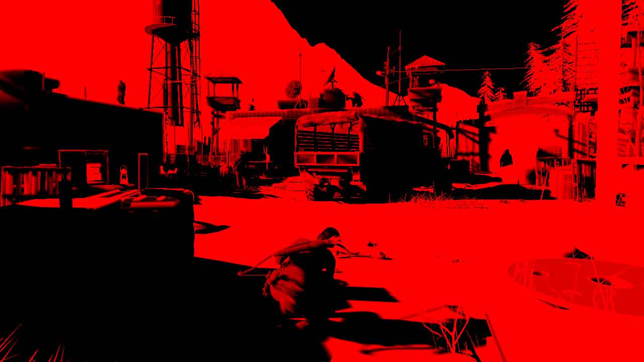
Analyzed frame
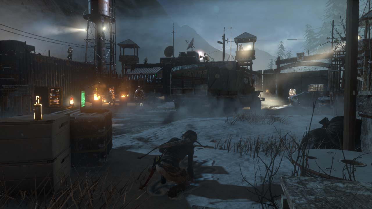
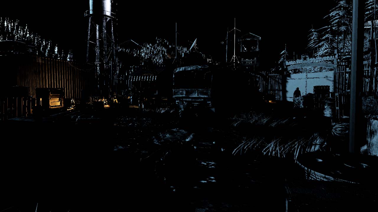
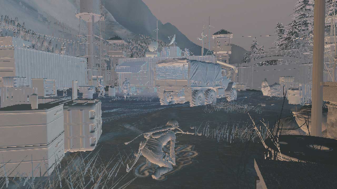
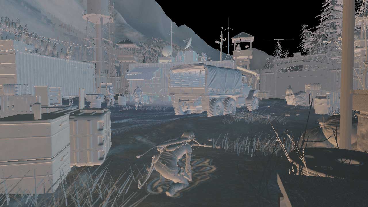
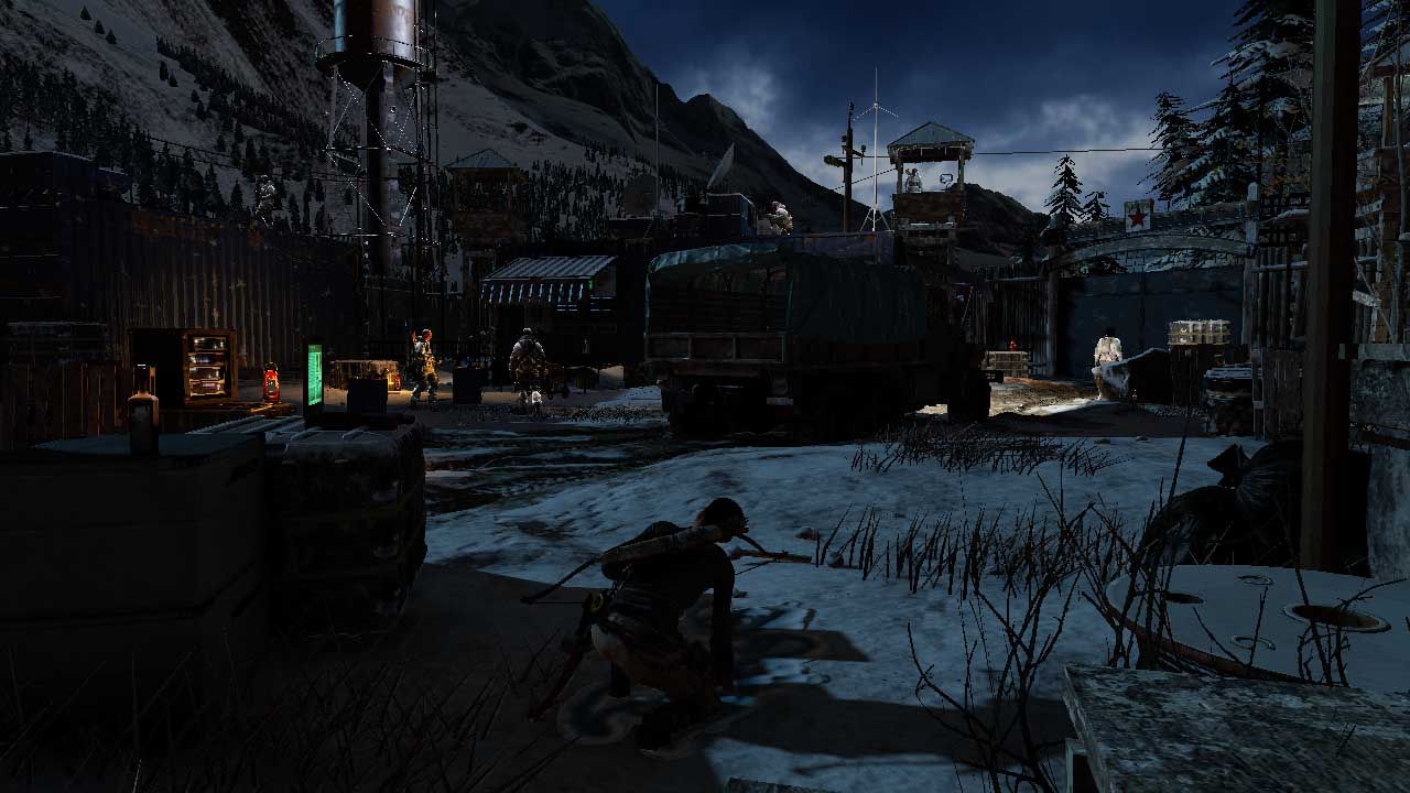
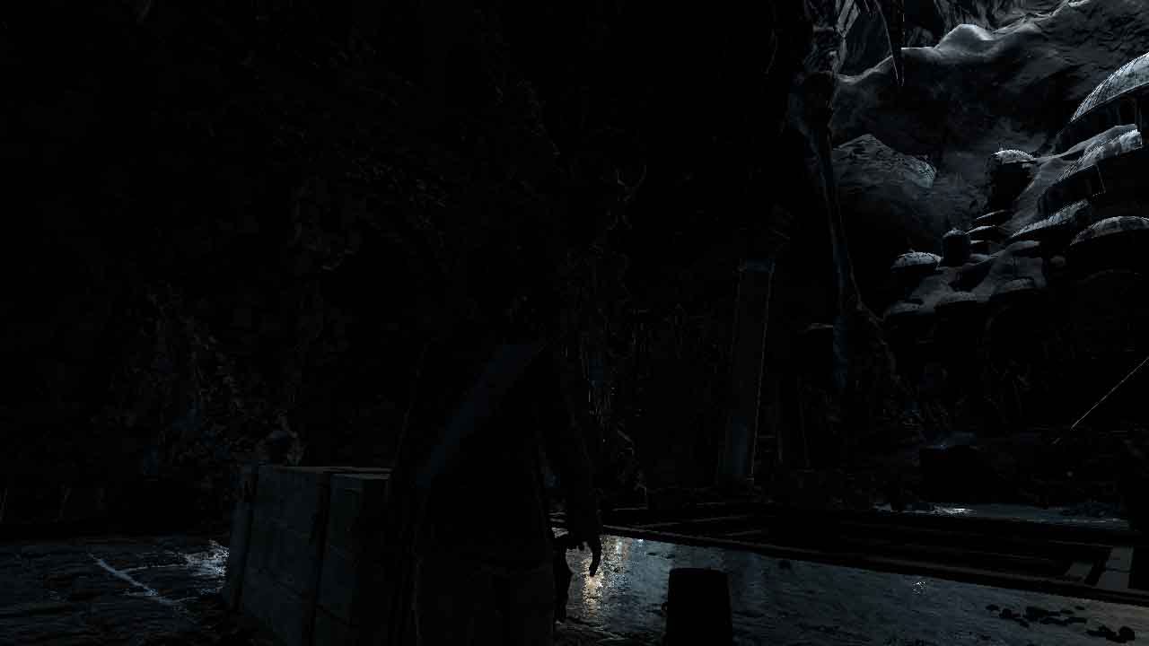
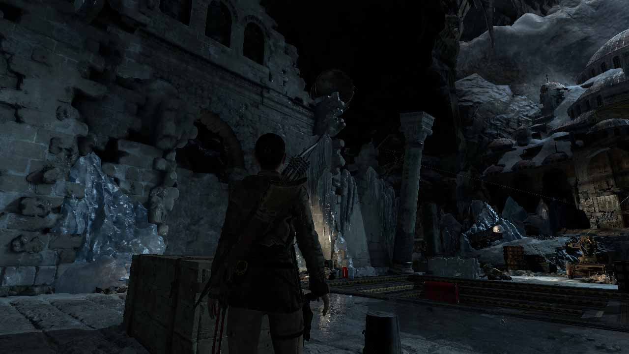
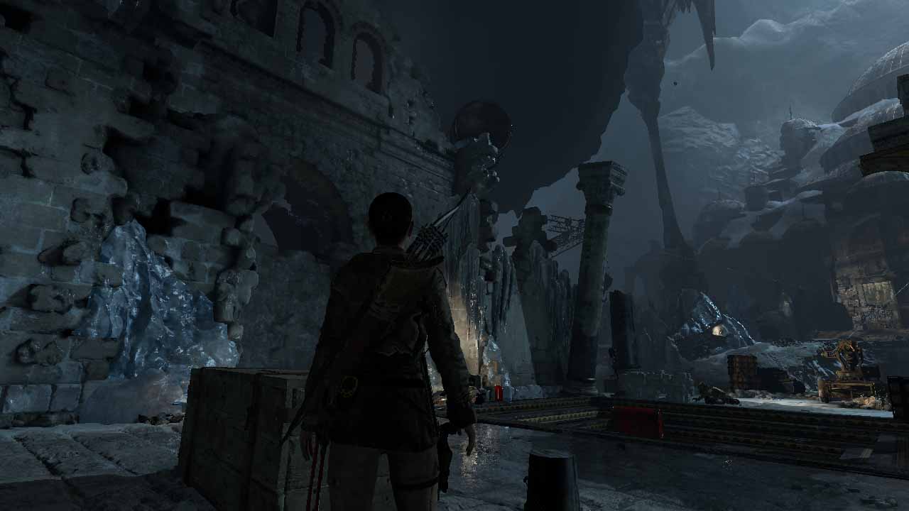
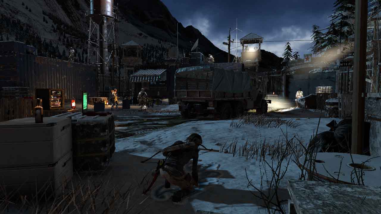
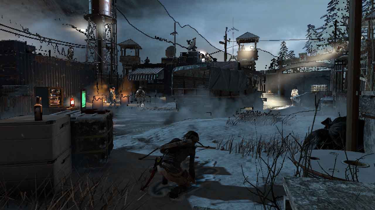
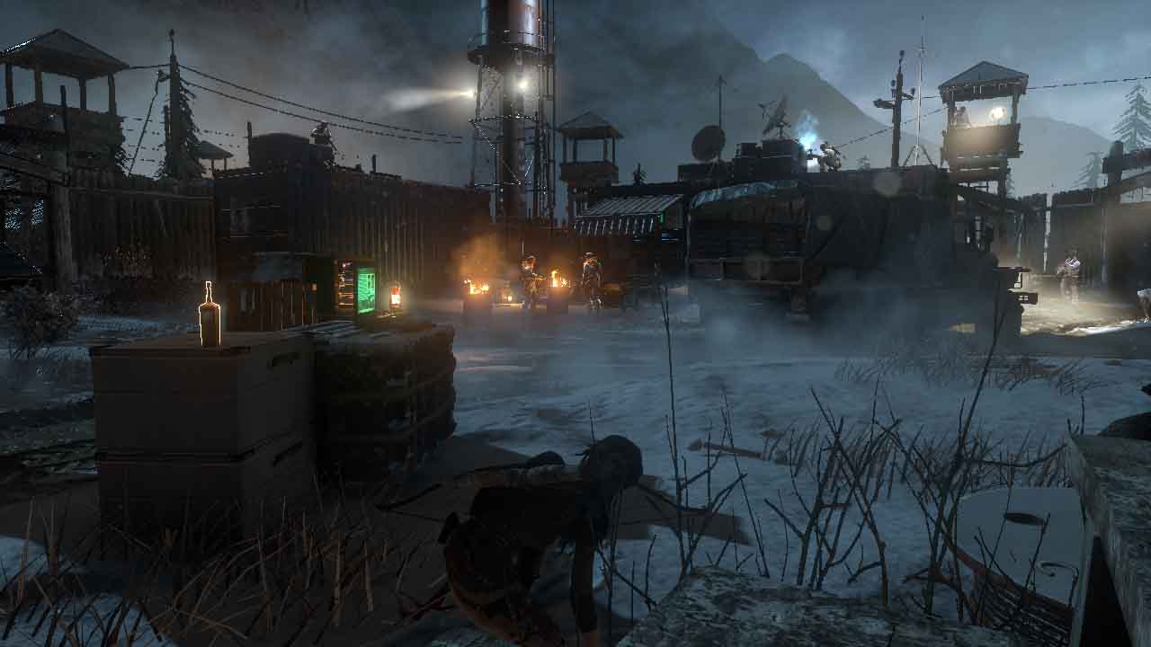
To avoid spoilers, I will say that in this frame the bad guys pursue Lara, because she is looking for an artifact that they are searching for. This conflict of interest does not resolve without weapons. Lara made her way to the enemy base at night. I chose a frame with atmospheric and contrasting lighting, in which the engine can show itself.
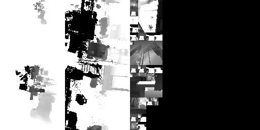
Preliminary depth pass
This is where the usual for many games optimization is performed - a small preliminary depth pass (approximately 100 draw calls). The game renders the largest objects (and not those that take up more space on the screen) to take advantage of the Early-Z video processors. Read more about it in an Intel article . In short, GPUs are able to avoid executing a pixel shader, if they can determine that it is covered by the previous pixel. This is a fairly low-cost pass, pre-filling the Z-buffer with depth values.
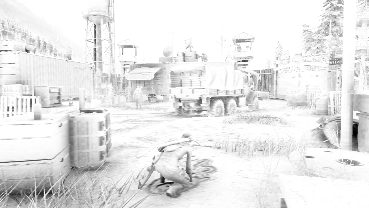
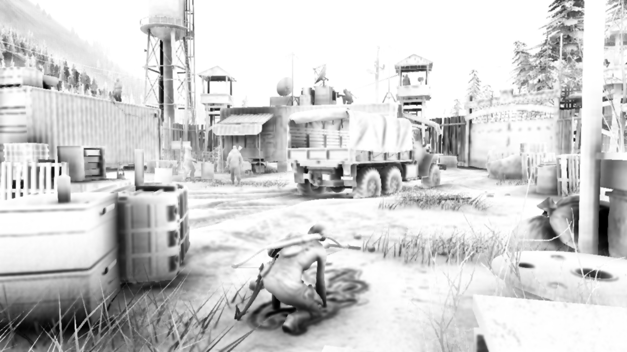
At this stage, I discovered an interesting technique of level of detail (LOD) called “fizzle” or “checkerboard”. This is a common way of gradually displaying or hiding objects at a distance in order to later either replace them with a lower-quality mesh, or completely hide them. Look at this truck. It seems that it is rendered twice, but in fact it is rendered with a high LOD and a low LOD in the same position. Each of the levels renders those pixels that the other did not render. The first LOD has 182226 vertices, and the second LOD has 47250. They are indistinguishable at a great distance, but one of them is three times less expensive. In this frame, LOD 0 almost disappears, and LOD 1 is rendered almost completely. After the complete disappearance of LOD 0, only LOD 1 will be rendered.

LOD 0
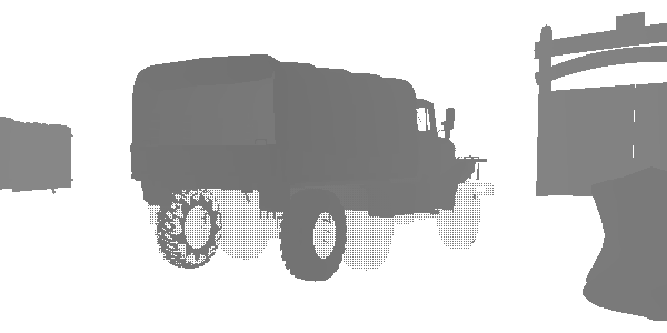
LOD 1
The pseudo-random texture and coefficient of probability allows us to discard pixels that do not pass the threshold value. This texture is used in the ROTR. One may wonder why not use alpha blending. Alpha blending has many drawbacks compared to fizzle fading.
- Convenience for the preliminary passage of the depths: thanks to the rendering of an opaque object with holes made in it, we can render in the preliminary passage and use early-z. Objects with alpha blending at this early stage are not rendered to the depth buffer due to sorting problems.
- The need for additional shaders : if a deferred renderer is used, then the shader of opaque objects does not contain any lighting. If you need to replace an opaque object with a transparent one, then a separate option is needed in which there is lighting. In addition to increasing the amount of memory required and the complexity due to at least one additional shader for all non-transparent objects, they must be accurate in order to avoid objects from protruding. This is difficult for many reasons, but it all comes down to the fact that rendering is now performed along a different code path.
- More redrawing : alpha blending can create a large redraw and, at a certain level of object complexity, a large portion of the bandwidth may be required to shade the LOD.
- Z-conflicts : Z-conflicts are a blink effect , when two polygons are rendered at a very close depth to each other. In this case, the inaccuracy of floating point calculations causes them to be rendered in turn. If we render two consecutive LODs, gradually hiding one and showing the second, they can cause a z-conflict, because they are very close to each other. There are always ways to get around this, for example, preferring one polygon to another, but such a system is difficult.
- Z-Buffer Effects : Many effects like SSAO use only a depth buffer. If we render transparent objects at the end of the pipeline, when ambient occlusion is already done, we could not take it into account.
The disadvantage of this technique is that it looks worse than alpha blending, but a good noise pattern, blurring after a fizzle or temporal anti-aliasing can almost completely hide it. In this regard, ROTR does not do anything particularly unusual.
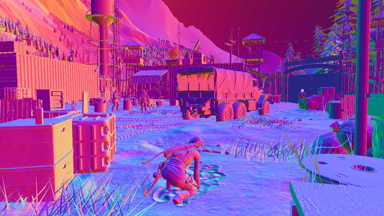
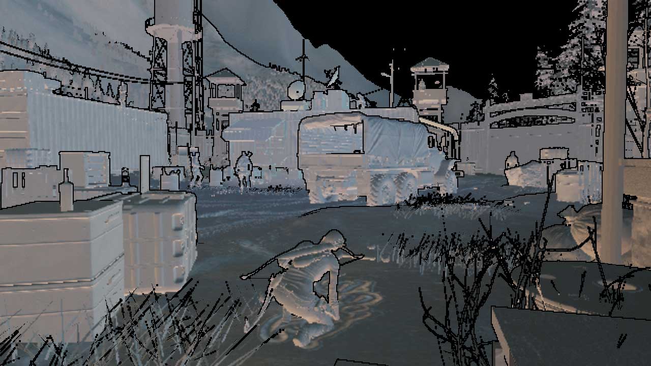
Normal pass
Crystal Dynamics uses a rather unusual lighting scheme in its games, which we will look at in the lighting aisle. For now, suffice it to say that the engine does not have a G-buffer pass; at least to the extent that is common in other games. On this pass, objects pass only depth and normal information to the output. Normals are written to the RGBA16_SNORM format render target in global space. It is curious that this engine uses the Z-up scheme, and not Y-up (the Z axis is directed upward, not Y), which is more often used in other engines / modeling packages. The alpha channel contains glossiness (glossiness), which is further unpacked as
exp2(glossiness * 12 + 1.0). The glossiness value can also be negative, because the sign is used as a flag indicating whether the surface is metallic. This can be seen independently, because all the dark colors in the alpha channel refer to metal objects.| R | G | B | |
| Normal.x | Normal.y | Normal.z | Glossiness + Metalness |
Normals

Glossiness / Metalness
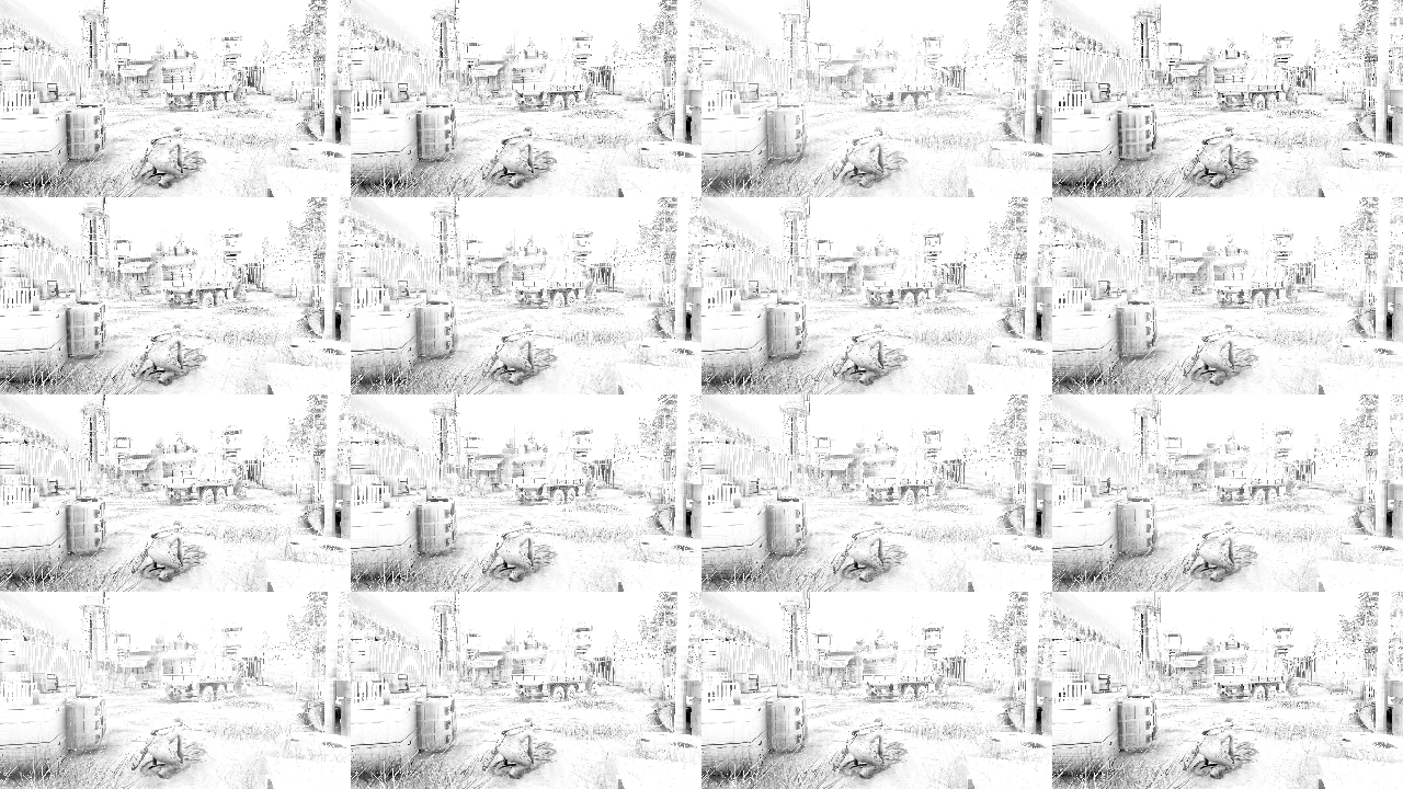
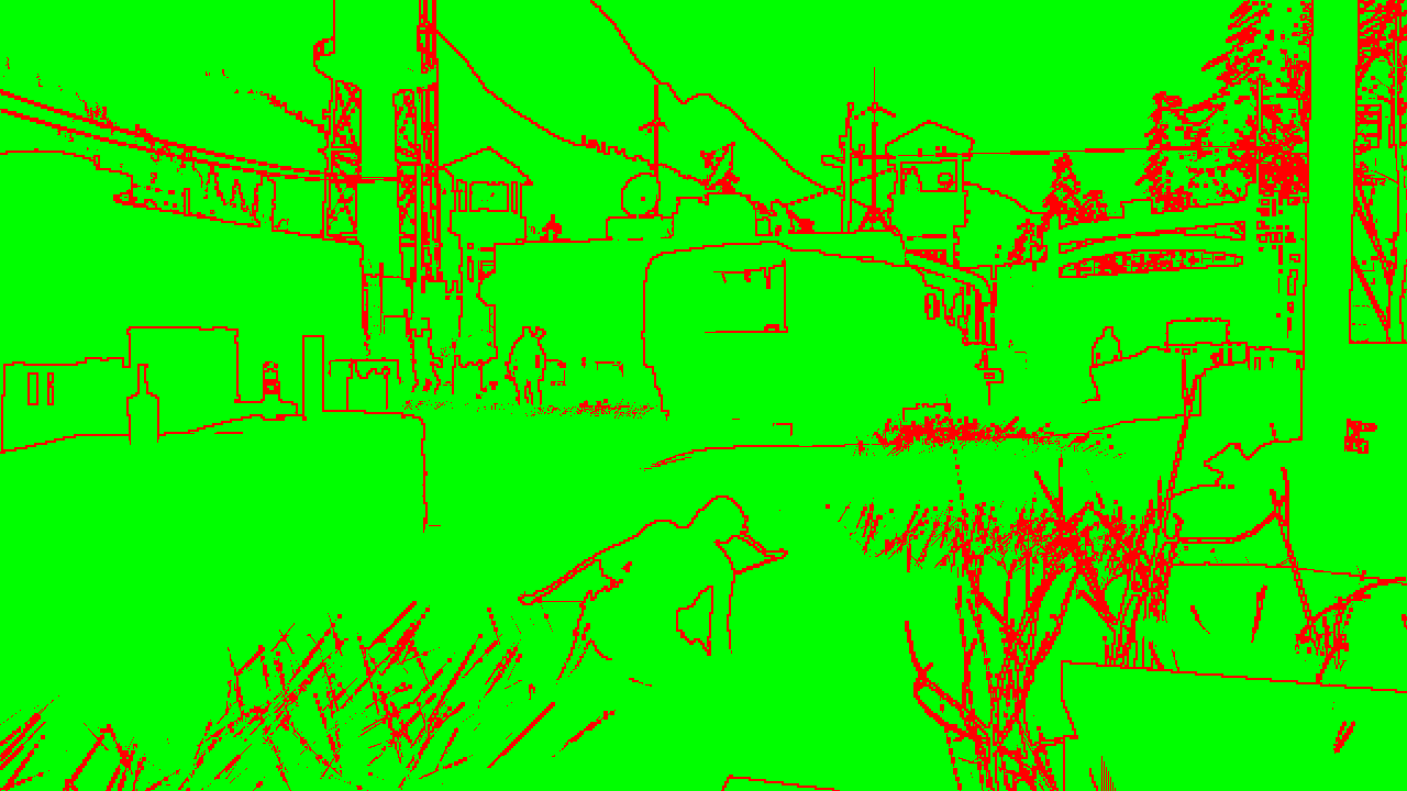
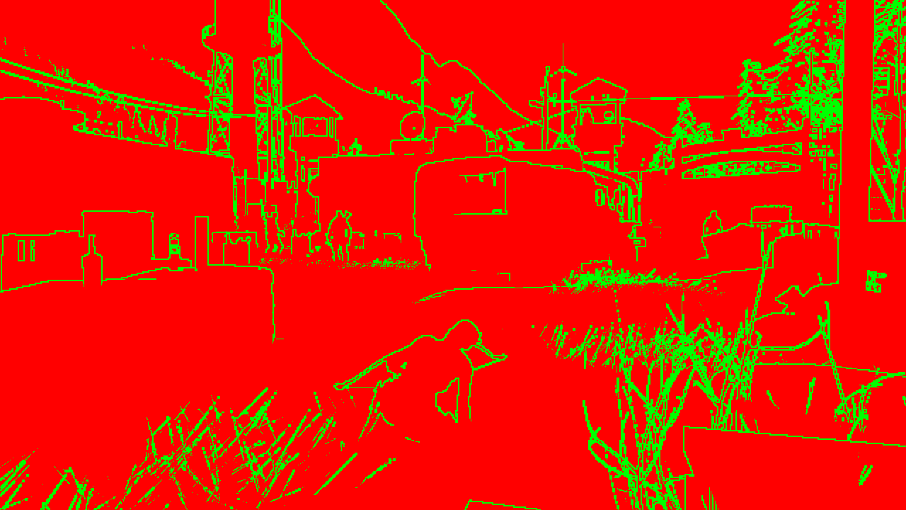
Benefits of Pre-Pass Depths

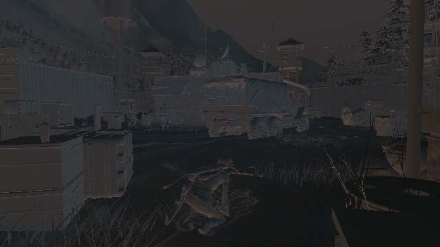
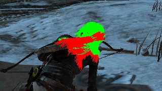
Remember that in the “Pre-Pass Depths” section, we talked about saving costs per pixel? I’ll go back a little to illustrate it. Take the following image. This is a rendering of the detailed part of the mountain to the normal buffer. Renderdoc kindly selected the pixels that passed the depth test, in green, and those that did not pass it - in red (they are not rendered). The total number of pixels that would be rendered without this preliminary pass is approximately 104518 (calculated in Photoshop). The total number of pixels actually rendered is 23858 (calculated by Renderdoc). Savings of about 77%! As we can see, with clever use, this preliminary pass can give a big win, but it requires only about a hundred draw calls.
Record multithreaded commands

It is worth noting one interesting aspect, because of which I chose the DX12 renderer - the recording of multi-threaded commands. In previous APIs, such as DX11, rendering is usually performed in a single thread. The graphics driver received rendering commands from the game and constantly transmitted requests to the GPU, but the game did not know when this would happen. This leads to inefficiency, because the driver must somehow guess what the application is trying to do and does not scale to multiple threads. Newer APIs, such as the DX12, take control of the developer, who can decide how to write commands and when to send them. Although Renderdoc cannot show how the recording is performed, you will see that there are seven color passes marked as Color Pass N, and each one is wrapped in a pair of ExecuteCommandList: Reset / Close. It marks the beginning and end of the list of commands. The list has about 100-200 draw calls. This does not mean that they were recorded using multiple streams, but hints at it.
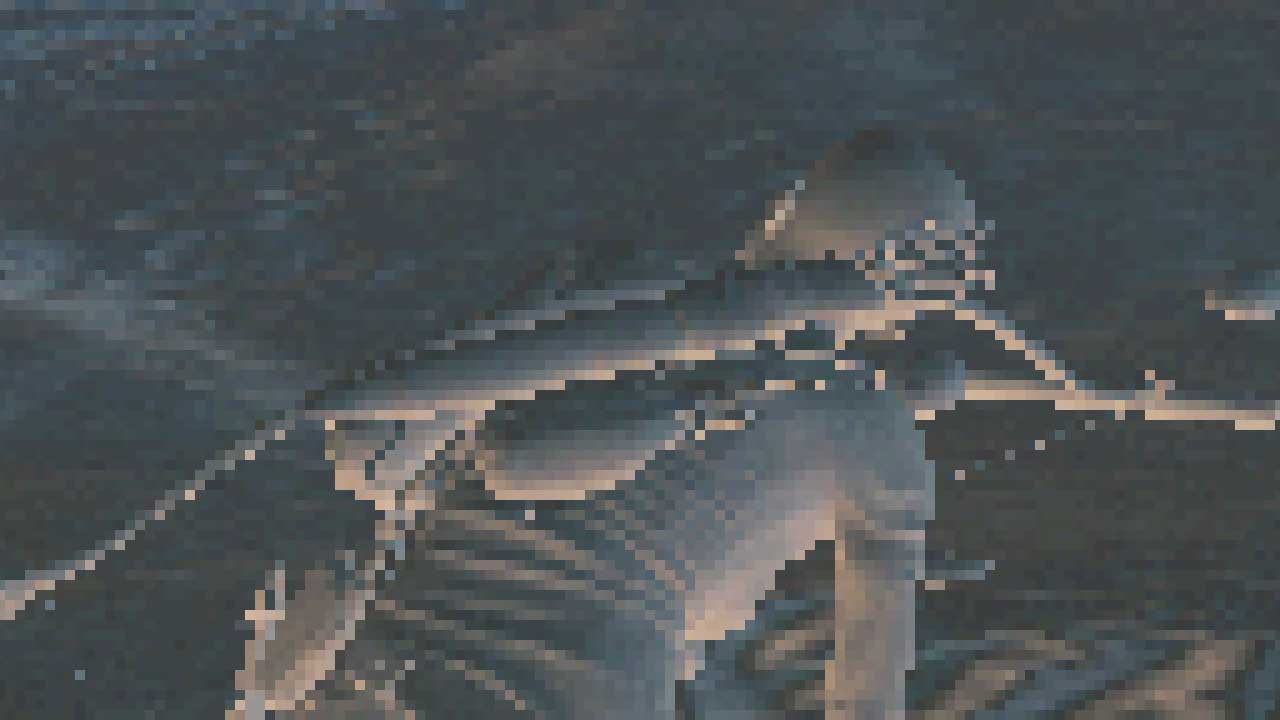
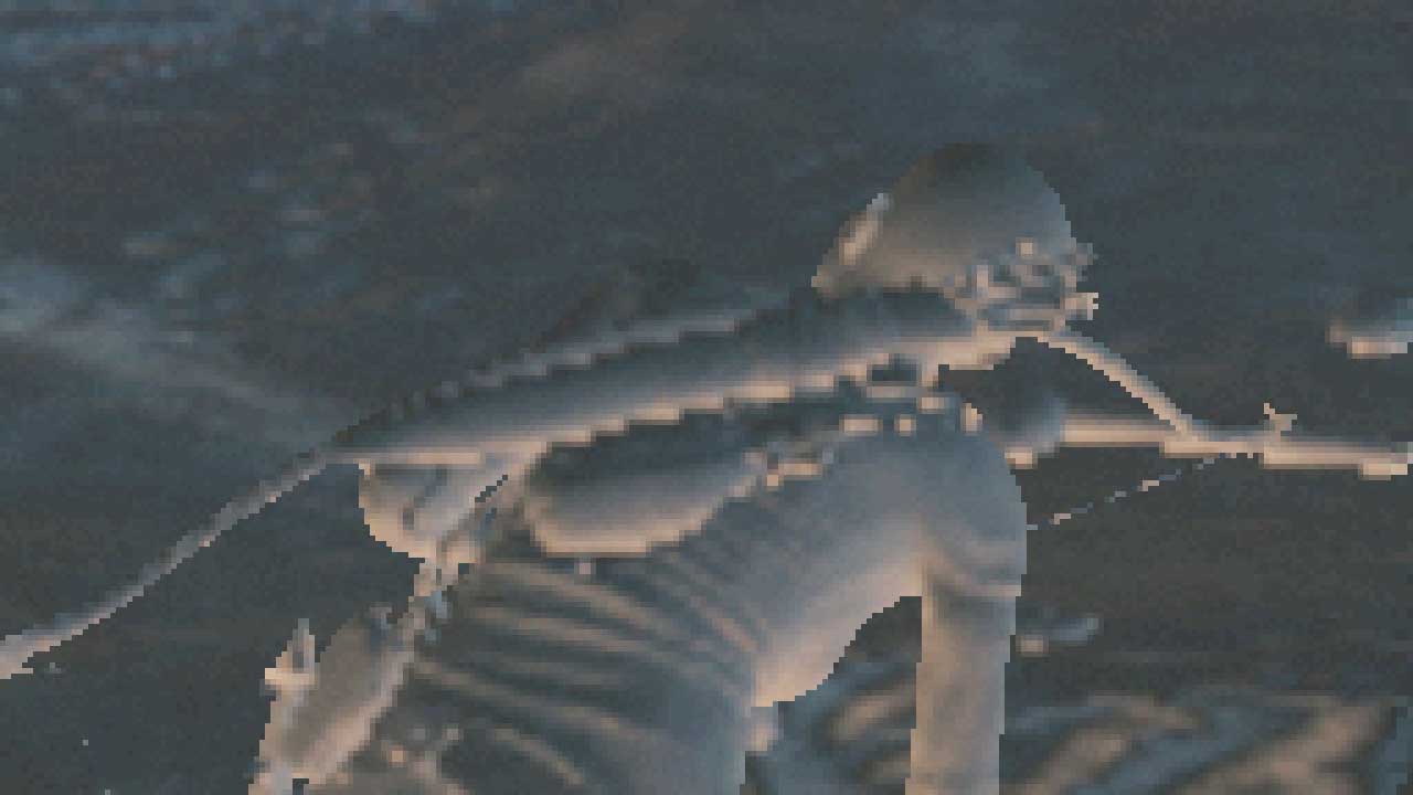
Footprints in the snow

If you look at Lara, you can see that when moving before the screenshot, she left traces in the snow. In each frame, a compute shader (compute shader) is executed, recording deformations in certain areas and applying them based on the type and height of the surface. Here, only the normal map is applied to the snow (i.e., the geometry does not change), but in some areas where the snow thickness is greater, the deformation is actually performed! You can also see how the snow “falls” into place and fills the traces left by Lara. Much more detail this technique is described in GPU Pro 7 . The snow deformation texture is a kind of height map that tracks Lara's movements and is glued along the edges so that the sampling shader can take advantage of this folding.
Shadow Atlas
When creating Shadow mapping, a fairly common approach is used - packing as many shadow maps as possible into the overall shadow texture. This shadow atlas is actually a huge 16-bit texture of 16384 × 8196. This makes it very flexible to reuse and scale the shadow maps that are in the atlas. In the frame we analyzed, 8 shadow maps were recorded in the atlas. Four of them are the main source of directional light (the moon, because it happens at night), because they use cascading shadow maps - fairly standard technique shadows long distances for directional lighting, which I have already explained a little earlier. More interestingly, several spotlights and spotlights are also included in the capture of this frame. The fact that 8 shadow maps are recorded in this frame does not mean that there are only 8 sources of the cast shadow of lighting. A game can cache shadow calculations, that is, lighting that has not changed either the position of the source or the geometry in the area of operation should not update its shadow map.
It seems that the rendering of shadow maps also benefits from writing multi-threaded commands to the list, and in this case, for the rendering of shadow maps, there are as many as 19 lists of commands.
Shadows from directional lighting
Shadows from directional lighting are calculated to the passage of lighting and later sampled. I do not know what would happen if there were several sources of directional lighting in the scene.
Ambient occlusion
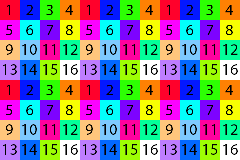
For ambient occlusion, ROTR allows you to use either HBAO or its HBAO + variant (this technique was originally published by NVIDIA). There are several variations of this algorithm, so I’ll look at the one I found in ROTR. First, the depth buffer is divided into 16 textures, each of which contains 1/16 of all depth values. Separation is performed in such a way that each texture contains one value from the 4 × 4 block of the original texture shown in the figure below. The first texture contains all the values marked in red (1), the second - the values marked in blue (2), and so on. If you want to know more about this technique, then here is the article by Louis Bavoil , who was also one of the authors of the HBAO article.
The next stage calculates for each texture ambient occlusion, which gives us 16 AO textures. The ambient occlusion is generated as follows: the depth buffer is sampled several times, recreating the position and accumulating the result of the calculations for each of the samples. Each ambient occlusion texture is calculated using different sampling coordinates, that is, in a 4 × 4 pixel block, each pixel tells its own part of the story. This is done for performance reasons. Each pixel already samples the depth buffer 32 times, and the full effect will require 16 × 32 = 512 samples, which is a brute force even for the most powerful GPUs. Then they are recombined into one full-screen texture, which turns out to be quite noisy, therefore, to smooth the results immediately after that, a passage of full-screen blur is performed. A very similar solution we saw inShadow of Mordor .
HBAO parts

Full HBAO with noise
Full HBAO with horizontal blur
Ready HBAO
Tile pre-lighting
Light Prepass is a rather unusual technique. Most development teams use a combination of deferred + direct lighting calculations (with variations, for example, with tile, clustered) or completely direct for some screen space effects. Technique pre-pass lighting is so unusual that it deserves an explanation. If the concept of traditional deferred lighting is to separate the properties of materials from the lighting, then the idea of separating the lighting from the properties of materials is at the heart of the preliminary lighting pass. Although this formulation looks a bit silly, the difference from traditional deferred lighting is that we store all the properties of materials (such as albedo, specular color, roughness, metalness, micro-occlusion, emissive) in a huge G-buffer, and use it later as input to subsequent light passes. Traditional deferred lighting may represent a large bandwidth load; the more complex the materials, the more information and operations are needed in the G-buffer. However, in the pre-pass lighting, we first accumulate all the lighting separately using the minimum amount of data, and then apply them in subsequent passes to the materials. In this case, illumination is sufficient only for normals, roughness and metalness. Shaders (two passes are used here) output data to three RGBA16F render targets. One contains diffuse illumination, the second is specular illumination, and the third is ambient illumination. At this stage, all shadow data is taken into account. Curious,here ). From this point of view, the entire frame is not complete.

Diffuse lighting
Mirror lighting
Ambient Lighting
Tile Optimization
Tile lighting is an optimization technique designed to render a large number of lighting sources. ROTR splits the screen into 16 × 16 tiles, and then stores information about which sources intersect each tile, that is, lighting calculations will be performed only for those sources that relate to tiles. At the beginning of the frame, a sequence of computational shaders is launched, determining which sources are related to tiles. At the lighting stage, each pixel determines which tile it is in and loops around each light source in the tile, performing all light calculations. If the binding of sources to tiles is done qualitatively, then you can save a lot of calculations and much of the bandwidth, as well as improve performance.
Scale up to depth
Depth based sampling is an interesting technique that is useful on this and subsequent passes. Sometimes computationally expensive algorithms cannot be rendered at full resolution, so they are rendered with a lower resolution, and then increase in scale. In our case, the ambient lighting is calculated at half the resolution, that is, after the calculations, the lighting must be correctly recreated. In its simplest form, 4 pixels of low resolution are taken and interpolated to get something resembling the original image. It works for smooth transitions, but it looks bad on discontinuities of surfaces, because there we mix quantities that are not related to each other, which may be adjacent in the screen space, but distant from each other in the global space. In solving this problem, several samples of the depth buffer are usually taken and compared with the sample of depths that we want to recreate. If the sample is too far, then we do not take it into account when recreating. Such a scheme works well, but it means that the reconstruction shader heavily loads the bandwidth.
ROTR makes a tricky move with the early dropping of stencil. After the passage of the normals, the depth buffer is completely filled, so the engine performs a full-screen passage that marks all discontinuous pixels in the stencil buffer. When it comes time to recreate the ambient lighting buffer, the slider uses two shaders: one is very simple for areas without depth gaps, the other is more complex for pixels with gaps. An early stencil discards pixels if they do not belong to the corresponding area, that is, there are costs only in the desired areas. The following images are much clearer:
Ambient lighting at half resolution
Increase the depth of the internal parts
Ambient lighting in full resolution, without edges
Edge Scale Increase
Ready ambient lighting
Approximate half resolution view
Approximate view of the recreated image
After the preliminary passage of the lighting, the geometry is transferred to the pipeline, only this time each object samples the lighting textures, the ambient occlusion texture and other material properties that we did not write to the G-buffer from the very beginning. This is good, because throughput is greatly saved here due to the fact that you don’t need to read a bunch of textures to write them into a large G-buffer, and then read them / decode them again. The obvious disadvantage of this approach is that all the geometry needs to be transferred anew, and the pre-pass lighting textures themselves represent a large load on throughput. I wondered why not use a lighter format for pre-pass lighting textures, for example R11G11B10F, but there is additional information in the alpha channel, therefore it would be impossible. Anyway, this is an interesting technical solution. At this stage, all opaque geometry is already rendered and lit. Note that light emitting objects such as the sky and laptop screen are included.
Reflections
This scene is not a particularly good example for showing reflections, so I chose another. The reflection shader is a fairly complex combination of cycles that can be reduced to two parts: one samples the cubic maps, and the other performs SSR (Screen space reflection - calculating reflections in the screen space); All this is done in a single pass and at the end is mixed, taking into account the coefficient that determines whether the SSR detected reflections (probably, the coefficient is not binary, but is a value in the interval [0, 1]). SSR works in a standard way for many games - repeatedly traces the depth buffer, trying to find the best intersection between the ray reflected by the shaded surface and another surface in some part of the screen. SSR works with the previously-scaled mip chain of the current HDR buffer, rather than the entire buffer.
There are also such adjustment factors as reflection brightness, as well as a kind of Fresnel texture, which was calculated before this passage, based on normals and roughness. I’m not completely sure, but after examining the assembler code, it seems to me that ROTR can calculate SSR only for smooth surfaces. There is no mip chain of blur in the engine after the SSR stage that exists in other engines , and there is not even anything like tracing the depth buffer using rays, which varies based on roughness. In general, rougher surfaces get reflections from cubic maps, or not at all. However, where SSR works, its quality is very high and stable, given that it does not accumulate over time and spatial blur is not performed for it. Alpha data also supports SSR (in some temples you can see very beautiful reflections in the water) and this is a good addition that you will not often see.

Reflections to
Reflection buffer

Reflections after
Illuminated fog

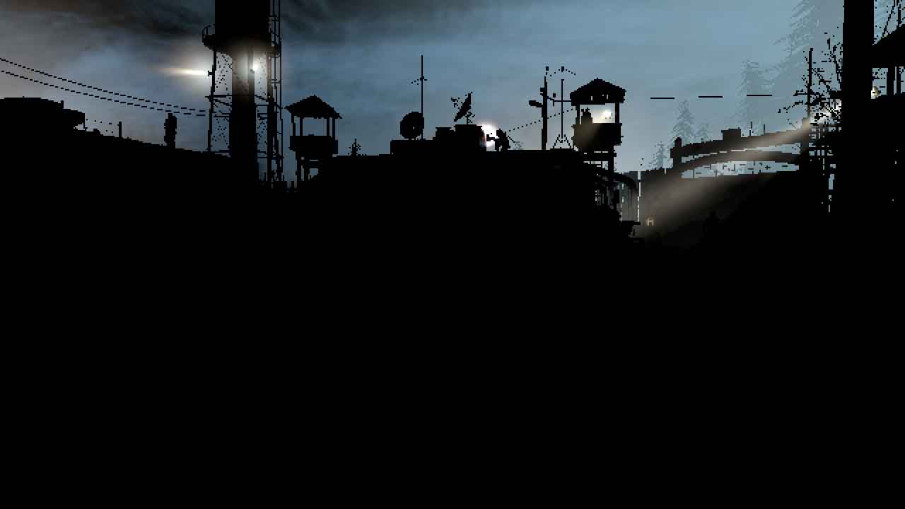
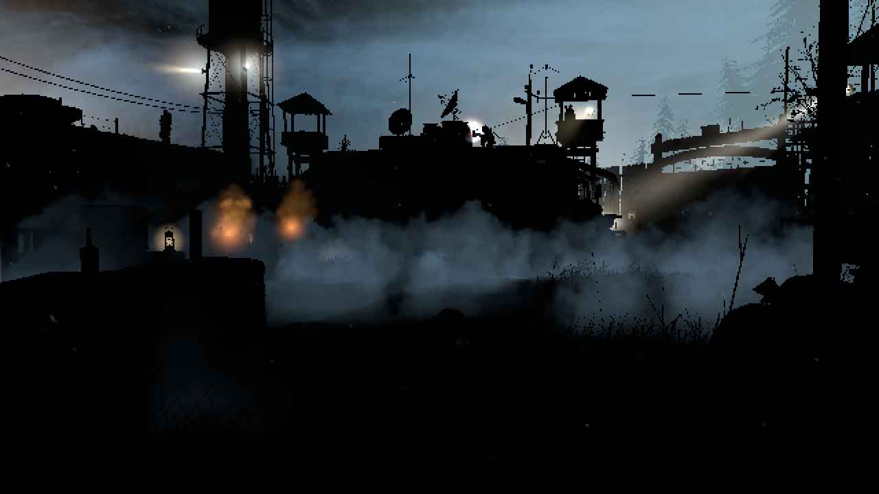
In our scene, fog is represented poorly because it darkens the background, and therefore is created by particles, so that we again use the reflection example. The fog is relatively simple, but quite effective. There are two modes: global, the overall color of the fog, and the color of the scatter inward, obtained from the cube map. Perhaps, the cubic map was again taken from the cubic reflection maps, or perhaps it was created anew. In both modes, the rarefaction of the fog is taken from the global rarefaction texture, in which the rarefaction curves are packed for several effects. In such a scheme, it is remarkable that it gives a very low-cost illuminated fog, i.e. Inward scattering changes in space, creating the illusion of mist interaction with distant illumination. This approach can also be used for atmospheric dispersion inside the sky.
Fog up
Fog after
Volumetric lighting
In the early stages of the frame, several operations take place to prepare for volumetric lighting. Two buffers are copied from the CPU to the GPU: the indices of the light sources and the data of the light sources. Both are read by a compute shader that outputs a 40x23x16 3D texture from a camera containing the number of light sources crossing this area. The texture is 40 × 23 in size because each tile is 32 × 32 pixels (1280/32 = 40, 720/32 = 22.5), and 16 is the number of pixels in depth. Not all light sources are included in the texture, but only those that are marked as voluminous (there are three in our scene). As we will see below, there are other fake volume effects created by flat textures. The displayed texture has a higher resolution - 160x90x64.
- The first pass determines the amount of light entering the cell within the volume in the form of a pyramid of visibility. Each cell accumulates the influence of all light sources, as if they have suspended particles that react to light and return part of it to the camera.
- The second pass blurs the lighting with a small radius. This is probably necessary to avoid flickering when moving the camera, because the resolution is very low.
- The third pass bypasses the volume texture from front to back, incrementally adding the influence of each source and giving the finished texture. In fact, it simulates the total amount of incoming light along the beam to a given distance. Since each cell contains a part of the world reflected by particles in the direction of the camera, in each of them we will get the joint contribution of all the cells that were previously traversed. This pass also performs a blur.
When all this is completed, we get a 3D texture that tells how much light a particular position gets relative to the camera. All that remains is to make a full-screen passage - to determine this position, find the corresponding voxel texture and add it to the HDR buffer. The lighting shader itself is very simple and contains only about 16 instructions.

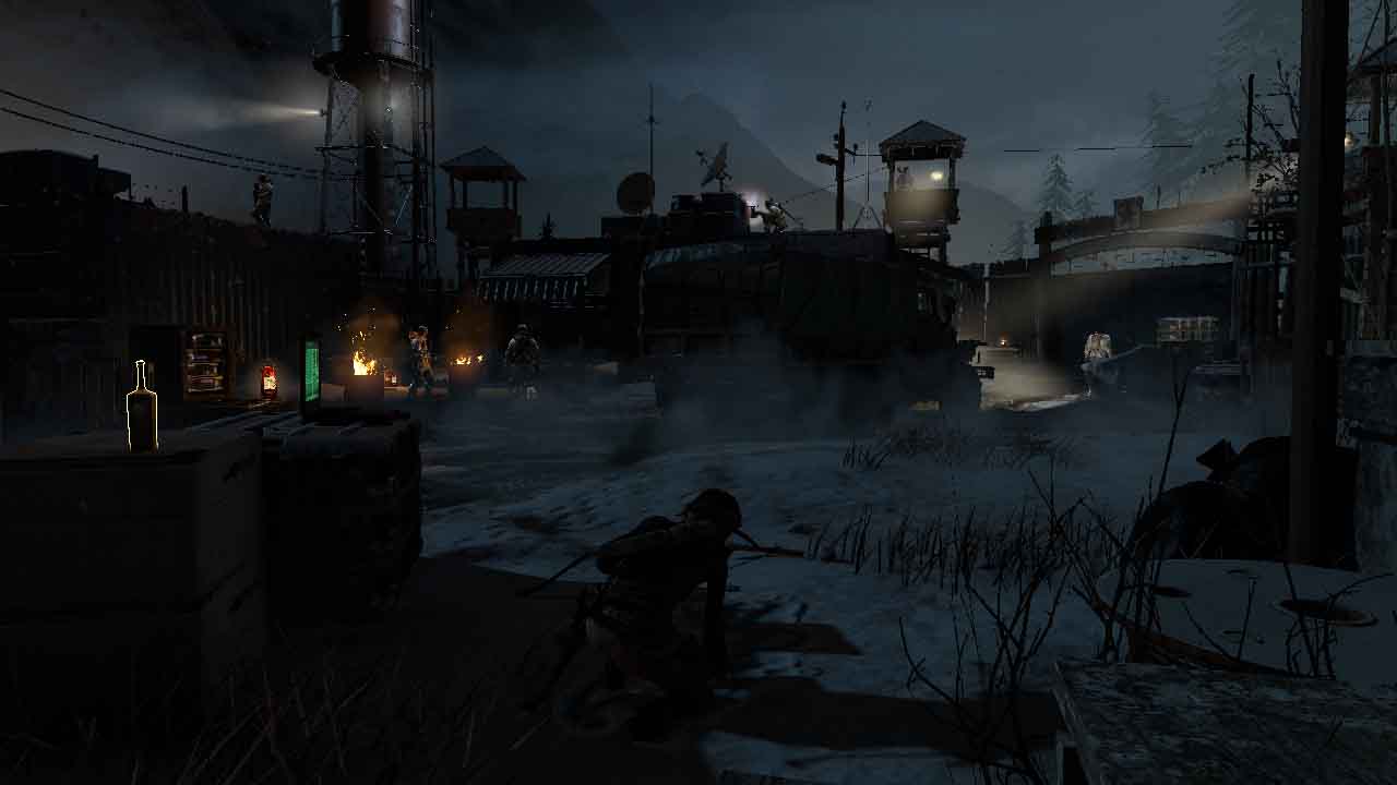
Volumetric lighting up to

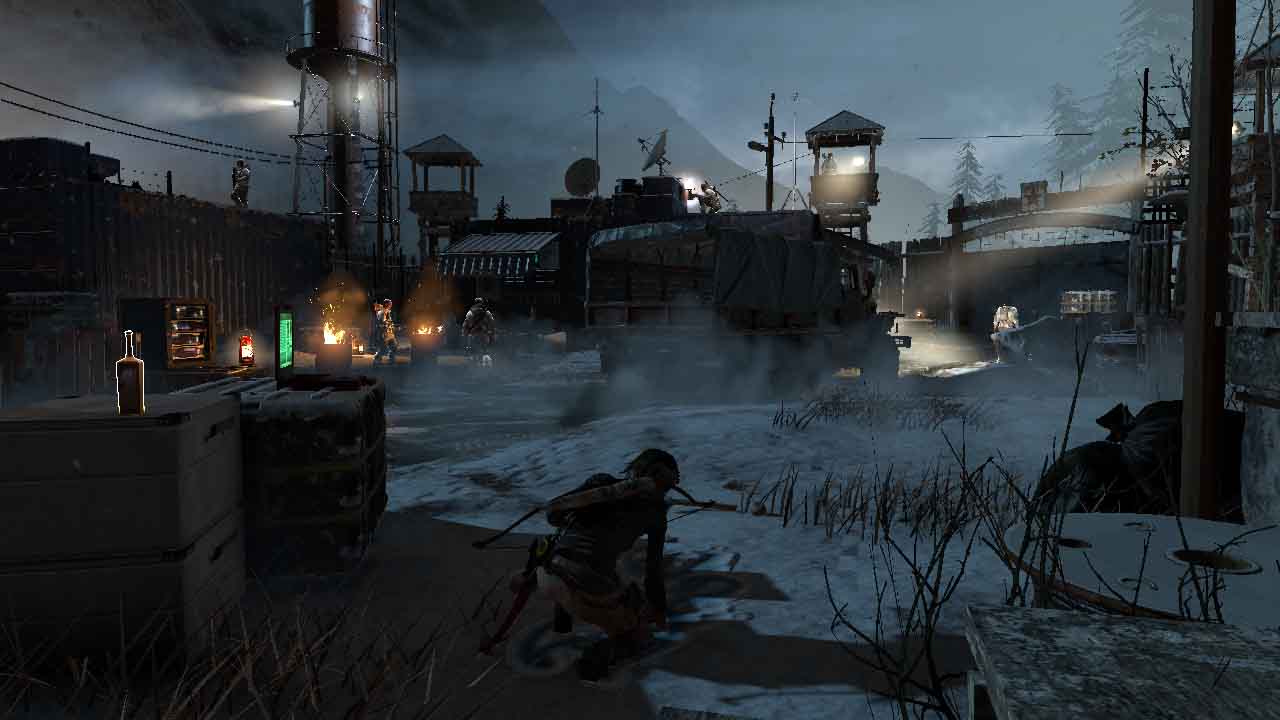
Bulk lighting after
Hair rendering
If the PureHair function is not turned on, then standard layers of hair are rendered on top of each other. This solution still looks great, but I would like to focus on the most advanced technologies. If the function is on, the frame starts with a simulation of Lara's hair by a sequence of computational heads. The first part of the Tomb Raider used a technology called TressFX, and in the sequel Crystal Dynamics implemented an improved technology. After the initial computation, as many as 7 buffers are obtained. All of them are used to control Lara's hair. The process is as follows:
- Run a compute shader to calculate motion values based on previous and current positions (for motion blur)
- Run a computational shader to populate a 1 × 1 cubic luminance map based on the reflection probe and luminosity information (illumination)
- Creating approximately 122 thousand vertices in the Triangle Strip mode (each strand of hair is a strip). There is no vertex buffer here, as you would expect with regular draw calls. Instead, there are 7 buffers containing everything needed to build hair. The pixel shader performs manual cropping; if the pixel is outside the window, it is discarded. This passage marks the stencil as "containing hair."
- The light / fog pass renders a full-screen quad with the stencil testing turned on so that only those pixels in which hair is actually visible are calculated. In fact, he considers hair as opaque and limits shading only to those strands that are visible on the screen.
- There is also a final pass, like step 4, which only displays the depth of the hair (it copies the hair depth from the texture)
If you are interested in learning more about this, then AMD has a lot of resources and presentations , because it is a public library created by the company . I was confused by the stage before stage 1, in which the same draw call is performed as in stage 3, while it says that it renders only depth values, but in fact the content is not rendered, and that is curious; maybe Renderdoc keeps back on me. I suspect that he may have tried to perform a conditional rendering request, but I do not see any prediction calls.

Hair up
Visible hair pixels

Hair shading
Tile rendering of alpha data and particles
Transparent objects again use the tile classification of light sources calculated for the tile pre-aisle lighting. Each transparent object calculates its own illumination in one pass, that is, the number of instructions and cycles becomes quite frightening (that is why a preliminary pass of illumination was used for non-transparent objects). Transparent objects can even perform reflections in screen space if they are on! Each object is rendered in the sort order from back to front, directly into the HDR buffer, including glass, flame, water in the tracks, etc. The alpha passage also renders edge highlighting when Lara focuses on an object (for example, on a bottle with a combustible mixture on a box on the left).
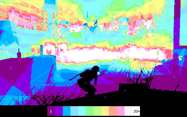
However, the particles are rendered into a half-resolution buffer to smooth out the huge load on the bandwidth created by their redrawing, especially when many large, screen-covering particles are used to create fog, haze, flames, etc. Therefore, the HDR buffer and the depth buffer are halved on each side, after which the particles begin to be rendered. Particles create a huge amount of redrawing, some pixels are shaded about 40 times. On the heat map you can see what I mean. Since the particles were rendered in half resolution, the same clever scaling trick is used here as in ambient lighting (gaps are marked in the stencil, the first pass renders the internal pixels, the second recreates the edges). You may notice that the particles are rendered before some other alpha effects, such as flame, shine, etc. This is necessary so that the alpha can be properly sorted for, for example, smoke. You can also notice that there are "volumetric" rays of light coming from security spotlights. They are added here, rather than being created at the stage of volumetric lighting. This is a low-cost but realistic way to create them at a great distance.

Only opaque objects
First alpha pass

Half resolution particles 1
Half resolution particles 2
Half-resolution particles 3
Scaling up the internal parts

Zoom edges

Full alpha data
Exposure and tone correction
ROTR performs shutter speed and tone correction in a single pass. However, although we usually assume that gamma correction occurs during tone correction, this is not the case here. There are many ways to implement excerpts, as we have seen in other games . The luminance calculation in ROTR is very interesting and requires almost no intermediate data or passes, so we will explain this process in more detail. The entire screen is divided into 64 × 64 tiles, after which the computation of groups (20, 12, 1) of 256 streams each starts to fill the entire screen. Each thread essentially performs the following task (below is pseudocode):
for(int i = 0; i < 16; ++i)
{
    uint2 iCoord = CalculateCoord(threadID, i, j); // Obtain coordinate
    float3 hdrValue = Load(hdrTexture, iCoord.xyz); // Read HDRfloat maxHDRValue = max3(hdrValue); // Find max componentfloat minHDRValue = min3(hdrValue); // Find min componentfloat clampedAverage = max(0.0, (maxHDRValue + minHDRValue) / 2.0);
    float logAverage = log(clampedAverage); // Natural logarithm
    sumLogAverage += logAverage;
}
Each group calculates the logarithmic sum of all 64 pixels (256 streams, each of which processes 16 values). Instead of storing an average value, it saves the sum and the number of actually processed pixels (not all groups will process exactly 64 × 64 pixels, because, for example, they can go beyond the edges of the screen). The shader wisely uses local stream storage to separate the amount; Each stream first works with 16 horizontal values, and then the individual streams summarize all these values vertically, and finally the control flow of this group (stream 0) adds the result and stores them all into the buffer. This buffer contains 240 elements, essentially giving us the average brightness of many areas of the screen. The subsequent command starts 64 threads that bypass all these values in the loop and add them, to get the final screen brightness. It also goes back from logarithm to linear units.
I do not have much experience with exposure techniques, but reading this post by Krzysztof Narkovic has clarified some things. Saving to an array of 64 elements is necessary for calculating the moving average, at which you can view the previous calculated values and smooth the curve in order to avoid very sharp changes in brightness, which create sharp changes in the shutter speed. This is a very complex shader and I have not yet figured out all its details, but the end result is the shutter value corresponding to the current frame.
After finding adequate shutter speeds, one pass performs the final shutter speed plus tonal correction. ROTR seems to use photographic tonal correction (Photographic Tonemapping), which explains the use of logarithmic averages instead of the usual averages. The tonal correction formula in the shader (after exposure) can be expanded as follows:


A brief explanation can be found here . I could not figure out why an additional division by Lm is needed, because it cancels the effect of multiplication. In any case, whitePoint is 1.0, so the process does not do very much in this frame, only the shutter speed changes the image. There is not even a limitation of the values within the LDR interval! It occurs during color correction, when the color cube indirectly limits values greater than 1.0.
Exposure to

Exposure after
Lens flare
The lens flare (Lens Flares) is rendered in an interesting way. A small preliminary pass calculates a 1xN texture (where N is the total number of glare elements that will be rendered as lens flare, in our case there are 28). This texture contains an alpha value for a particle and some other unused information, but instead of calculating it from a visibility query or something like that, the engine calculates it by analyzing the depth buffer around the particle in the circle. For this, information about vertices is stored in a buffer accessible to the pixel shader.

Each element is then rendered as simple planes aligned with the screen, emitted from light sources. If the alpha value is less than 0.01, then the position is assigned the value NaN so that this particle is not rasterized. They are a bit like the bloom effect and add glow, but this effect itself is created later.
Lens flares up

Lens Flare Elements

Lens flares after
Bloom
Bloom uses a standard approach: downsampling of the HDR buffer is performed, bright pixels are isolated, and then their scale increases sequentially with blurring to expand their area of influence. The result is increased to the screen resolution and compositing is superimposed on top of it. There are a couple of interesting points worth exploring. The whole process is performed using 7 computational shaders: 2 for downsampling, 1 for simple blur, 4 for zooming in.
- The first downsampling from full to half resolution selects pixels brighter than a predetermined threshold value and outputs them to the target half resolution (mip 1). He also takes the opportunity and simultaneously performs a blur. You may notice that the first mip-texture becomes only slightly darker, because we have dropped pixels with a rather low threshold value of 0.02.
- The next downsampling shader takes a mip and creates mip 2, 3, 4 and 5 in one pass.
- The next pass in one pass blurs mip 5. There are no separable blur operations in the whole process that we have sometimes encountered. All blurring operations use group shared memory so that the shader takes as few samples as possible and reuses the data of its neighbors.
- Scaling up is also an interesting process. These 3 scale-ups use the same shader and take two textures, a previously blurred mip N and not a blurred mip N + 1, mixing them together with the coefficient transmitted from the outside, at the same time blurring them. This allows you to add more accurate details in the bloom instead of those that may disappear when blurring.
- The final zoom in increases mip 1 and adds it to the final HDR buffer, multiplying the result by the controlled power of bloom.

Bloom up

MIP 1 reduced scale bloom

MIP 2 reduced scale bloom

MIP 3 reduced scale bloom

MIP 4 reduced scale bloom
MIP 5 reduced scale bloom

Blur MIP 5 Bloom Effect

MIP 4 Zoom Bloom

MIP 3 Zoom Bloom
MIP 2 Zoom Bloom

MIP 1 Zoom Bloom

Bloom after The
curious aspect is that the reduced-scale textures change the aspect ratio. For the sake of visualization, I corrected them, and I can only guess at the reasons for this; Perhaps this is done so that texture sizes are multiple of 16. Another interesting point: since these shaders are usually very limited in bandwidth, the values stored in the group shared memory are converted from float32 to float16! This allows the shader to exchange math operations for doubling free memory and bandwidth. For this to become a problem, the range of values must be quite large.
FXAA
ROTR supports a wide range of various anti-aliasing techniques, such as FXAA (Fast Approximate AA) and SSAA (Super Sampling AA). Notable is the absence of the option to enable temporal AA, because for most modern AAA games it becomes standard. Be that as it may, FXAA copes with its task remarkably, SSAA also works well, this is a rather “hard” option if the game lacks performance.
Motion blur
Motion blur seems to use an approach very similar to the Shadows of Mordor solution.. After rendering the volumetric illumination, a separate rendering pass outputs motion vectors from animated objects to the motion buffer. This buffer is then combined with the motion caused by the camera, and the final motion buffer becomes the input to the blur pass, which blurs in the direction indicated by the motion vectors of the screen space. To estimate the blur radius for several passes, the texture of motion vectors is calculated on a reduced scale, so that each pixel has an approximate idea of what movement occurs next to it. Blur is performed in several passes at half resolution and, as we have seen, later its scale is enlarged in two passes using stencil. Multiple passes are performed for two reasons: first, to reduce the amount of texture reading required to create a blur with a potentially very large radius, and secondly, because different types of blur are performed. It depends on whether there is an animated character on the current pixels.
Motion blur up

Speed motion blur

Motion blur pass 1

Motion blur pass 2

Motion blur, pass 3

Motion blur, pass 4

Motion blur, pass 5

Motion blur, passage 6

Motion Blur, Zooming Internal Parts

Motion blur, zooming in on edges
Additional features and details
There are a few more things worth mentioning without much detail.
- Camera freeze: in cold weather adds snowflakes and frost to the camera
- Dirty camera: adds dirt to the camera
- Color Correction: A small color correction is performed at the end of the frame, using a fairly standard color cube to perform color correction, as described above, and also adds noise to give some scenes a severity.
Ui
The UI is implemented a bit unusual - it renders all elements in a linear space. Usually, by the time of rendering, the UI has already completed tonal correction and gamma correction. However, ROTR uses linear space right up to the very end of the frame. This makes sense, because the game uses a reminiscent 3D UI; however, before writing sRGB images to HDR buffer, they need to be converted to linear space so that the most recent operation (gamma correction) does not distort colors.
Let's sum up
I hope you enjoyed reading this analysis just as I created it. Personally, I definitely learned a lot from him. Congratulations to the talented developers from Crystal Dynamics for the fantastic work done to create this engine. I also want to thank Baldur Karlsson for his fantastic work on Renderdoc. His work made debugging graphics on a PC a much more convenient process. I think the only thing that was a little difficult in this analysis is tracking the shader launches themselves, because at the time of writing this article this function is not available for DX12. I hope, in time, she will appear and we will all be very pleased.