Neural Network Architecture
- Transfer
Translation Neural Network Architectures
Deep neural network algorithms have gained great popularity today, which is largely ensured by the well-thought-out architecture. Let's look at the history of their development over the past few years. If you are interested in a deeper analysis, refer to this work .
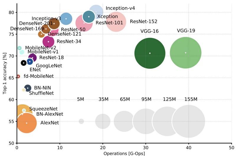
Comparison of popular architectures for Top-1 one-crop accuracy and the number of operations required for one direct pass. More details here .
In 1994, one of the first convolutional neural networks was developed, which laid the foundation for deep learning. This pioneering work by Yann LeCun, after many successful iterations since 1988, was called LeNet5 !

The LeNet5 architecture has become fundamental to deep learning, especially in terms of the distribution of image properties throughout the picture. Convolutions with learning parameters allowed using several parameters to efficiently extract the same properties from different places. In those years, there were no video cards that could speed up the learning process, and even the central processors were slow. Therefore, the key advantage of the architecture was the ability to save parameters and calculation results, in contrast to using each pixel as separate input data for a large multilayer neural network. In LeNet5, pixels are not used in the first layer, because images are strongly spatially correlated, so using individual pixels as input properties will not allow you to take advantage of these correlations.
Features of LeNet5:
This neural network formed the basis of many subsequent architectures and inspired many researchers.
From 1998 to 2010, the neural networks were in a state of incubation. Most people did not notice their growing capabilities, although many developers gradually honed their algorithms. Thanks to the heyday of mobile phone cameras and the cheapening of digital cameras, more and more training data has become available to us. At the same time, computing capabilities grew, processors became more powerful, and video cards turned into the main computing tool. All these processes allowed the development of neural networks, albeit rather slowly. Interest in tasks that could be solved with the help of neural networks was growing, and finally the situation became obvious ...
In 2010, Dan Claudiu Ciresan and Jurgen Schmidhuber published one of the first descriptions of the implementation of GPU neural networks . Their work contained the direct and reverse implementation of a 9-layer neural network on the NVIDIA GTX 280 .
In 2012, Alexei Krizhevsky published AlexNet , an in-depth and extended version of LeNet, which won by a wide margin in the ImageNet competition.
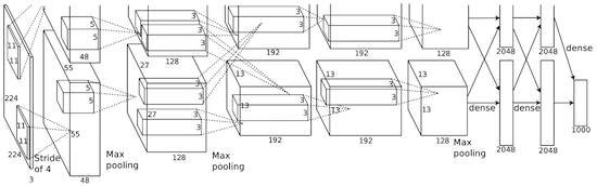
At AlexNet, the results of LeNet calculations are scaled into a much larger neural network, which is able to study much more complex objects and their hierarchies. Features of this solution:
By that time, the number of cores in video cards had grown significantly, which allowed them to reduce the training time by about 10 times, and as a result it became possible to use much larger datasets and pictures.
The success of AlexNet launched a small revolution, convolutional neural networks turned into a workhorse of deep learning - this term now means "large neural networks that can solve useful problems."
In December 2013, the NYU laboratory of Jan Lekun published a description of Overfeat , a variant of AlexNet. Also, the article described the trained bounding boxes, and subsequently many other works on this topic were published. We believe that it is better to learn how to segment objects, rather than using artificial bounding boxes.
In VGG networks developed at Oxford, in each convolutional layer, for the first time, 3x3 filters were used, and even these layers were combined in a sequence of convolutions.
This contradicts the principles laid down in LeNet, according to which large convolutions were used to extract the same image properties. Instead of the 9x9 and 11x11 filters used in AlexNet, much smaller filters began to be used, dangerously close to 1x1 convolutions, which LeNet authors tried to avoid, at least in the first layers of the network. But the great advantage of VGG was the finding that several 3x3 convolutions combined in a sequence can emulate larger receptive fields, for example, 5x5 or 7x7. These ideas will later be used in the Inception and ResNet architectures.
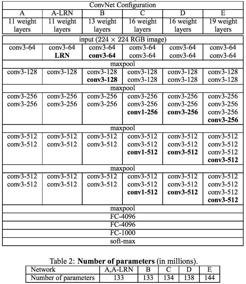
VGG networks use multiple 3x3 convolutional layers to represent complex properties. Pay attention to blocks 3, 4 and 5 in VGG-E: to extract more complex properties and combine them, 256 × 256 and 512 × 512 3 × 3 filter sequences are used. This is equivalent to a large convolutional classifier 512x512 with three layers! This gives us a huge number of parameters and excellent learning abilities. But it was difficult to learn such networks; I had to break them into smaller ones, adding layers one by one. The reason was the lack of effective ways to regularize models or some methods of limiting a large search space, which is promoted by many parameters.
VGG in many layers use a large number of properties, so training was computationally expensive. The load can be reduced by reducing the number of properties, as is done in the bottleneck layers of the Inception architecture.
The Network-in-network (NiN) architecture is based on a simple idea: using 1x1 convolutions to increase the combinatoriality of properties in convolutional layers.
In NiN, after each convolution, spatial MLP layers are used to better combine the properties before feeding to the next layer. It may seem that the use of 1x1 convolutions contradicts the original LeNet principles, but in reality it allows combining properties better than just stuffing more convolutional layers. This approach is different from using bare pixels as input for the next layer. In this case, 1x1 convolutions are used for spatial combination of properties after convolution within the framework of property maps, so you can use much fewer parameters that are common to all pixels of these properties!
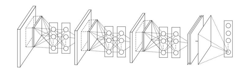
MLP can greatly increase the effectiveness of individual convolutional layers by combining them into more complex groups. This idea was later used in other architectures, such as ResNet, Inception, and their variants.
Google Christian Szegedy is worried about lowering computations in deep neural networks, and as a result created GoogLeNet, the first Inception architecture .
By the fall of 2014, deep learning models had become very useful in categorizing image content and frames from videos. Many skeptics have recognized the benefits of deep learning and neural networks, and Internet giants, including Google, have become very interested in deploying efficient and large networks on their server capacities.
Christian was looking for ways to reduce the computational load in neural networks, achieving the highest performance (for example, in ImageNet). Or preserving the amount of computation, but still increasing productivity.
As a result, the command created an Inception module:

At first glance, this is a parallel combination of convolutional filters 1x1, 3x3 and 5x5. But the highlight was the use of convolution blocks 1x1 (NiN) to reduce the number of properties before serving in the "expensive" parallel blocks. Usually this part is called bottleneck, it is described in more detail in the next chapter.
GoogLeNet uses a stem without Inception modules as the initial layer, and also uses average pooling and a softmax classifier similar to NiN. This classifier performs extremely few operations compared to AlexNet and VGG. It also helped create a very efficient neural network architecture .
This layer reduces the number of properties (and therefore operations) in each layer, so that the speed of obtaining the result can be maintained at a high level. Before transferring data to “expensive” convolutional modules, the number of properties is reduced, say, 4 times. This greatly reduces the amount of computation, which has made the architecture popular.
Let's figure it out. Suppose we have 256 properties at the input and 256 at the output, and let the Inception layer perform only 3x3 convolutions. We get 256x256x3x3 convolutions (589,000 operations of accumulation multiplication, that is, MAC operations). This may go beyond our computational speed requirements; let's say a layer is processed in 0.5 milliseconds on Google Server. Then reduce the number of properties for folding to 64 (256/4). In this case, we first perform a 1x1 convolution of 256 -> 64, then another 64 convolution in all Inception branches, and then again apply a 1x1 convolution of 64 -> 256 properties. Number of operations:
Only about 70,000, reduced the number of operations by almost 10 times! But at the same time, we did not lose generalization in this layer. Bottleneck layers have shown excellent performance on the ImageNet dataset, and have been used in later architectures such as ResNet. The reason for their success is that the input properties are correlated, which means that you can get rid of redundancy by correctly combining properties with 1x1 convolutions. And after folding with fewer properties, you can again deploy them into a significant combination on the next layer.
Christian and his team have proven to be very effective researchers. In February 2015, the Batch-normalized Inception architecture was introduced as the second version of Inception . Batch-normalization calculates the mean and standard deviation of all property distribution maps in the output layer, and normalizes their responses with these values. This corresponds to the "whitening" of the data, that is, the responses of all neural maps lie in the same range and with a zero mean. This approach makes learning easier, because the next layer is not required to remember offsets of input data and can only search for the best combinations of properties.
In December 2015, a new version of Inception modules and the corresponding architecture was released. The author’s article better explains the original GoogLeNet architecture, which tells much more about the decisions made. Key ideas:
Inception uses the pooling layer with softmax as the final classifier.
In December 2015, at about the same time that the Inception v3 architecture was introduced, a revolution occurred - they published ResNet . It contains simple ideas: submit the output of two successful convolutional layers And bypass the input for the next layer!

Such ideas have already been proposed, for example, here . But in this case, the authors bypass TWO layers and apply the approach on a large scale. Bypassing one layer does not give much benefit, and bypassing two is a key find. This can be seen as a small classifier, as network-in-network!
It was also the first ever example of training a network of several hundred, even thousands of layers.
Multilayer ResNet used a bottleneck layer similar to that used in Inception:

This layer reduces the number of properties in each layer, first using a 1x1 convolution with a smaller output (usually a quarter of the input), then a 3x3 layer, and then again convolving 1x1 into a larger number of properties. As in the case of Inception modules, this saves computational resources while maintaining a wealth of property combinations. Compare with the more complex and less obvious stems in Inception V3 and V4.
ResNet uses a pooling layer with softmax as the final classifier.
Every day, additional information about the ResNet architecture appears:
Christian and his team excelled again with a new version of Inception .
The Inception-module that comes after stem is the same as in Inception V3:

In this case, the Inception-module is combined with the ResNet-module:

This architecture turned out, to my taste, more complicated, less elegant, and also filled with opaque heuristic solutions. It is difficult to understand why the authors made these or those decisions, and it is equally difficult to give them any kind of assessment.
Therefore, the prize for a clean and simple neural network, easy to understand and modify, goes to ResNet.
SqueezeNet published recently. This is a remake in a new way of many concepts from ResNet and Inception. The authors demonstrated that improving the architecture reduces network size and the number of parameters without complex compression algorithms.
All the features of recent architectures are combined into a very efficient and compact network, using very few parameters and computing power, but at the same time giving excellent results. The architecture was called ENet , it was developed by Adam Paszke ( Adam Paszke ). For example, we used it for very accurate marking of objects on the screen and parsing scenes. A few examples of Enet . These videos are not related to the training dataset .
HereYou can find the technical details of ENet. It is a network based on encoder and decoder. The encoder is built on the usual CNN categorization scheme, and the decoder is an upsampling netowrk designed for segmentation by spreading the categories back to the original size image. For image segmentation, only neural networks were used, no other algorithms.
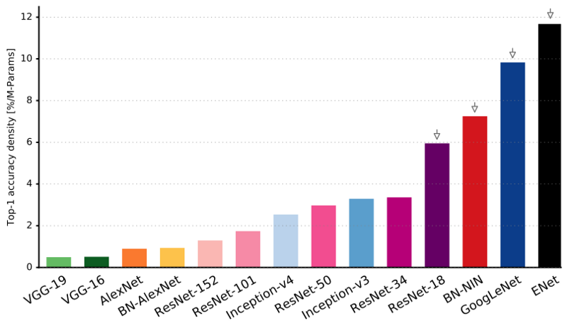
As you can see, ENet has the highest specific accuracy compared to all other neural networks.
ENet was designed to use as few resources as possible from the very beginning. As a result, the encoder and decoder together occupy only 0.7 MB with fp16 precision. And with such a tiny size, ENet is not inferior to segmentation accuracy or superior to other purely neural network solutions.
Published a systematic assessment of CNN modules. It turned out to be beneficial:
Xception introduced a simpler and more elegant architecture into the Inception module, which is no less efficient than ResNet and Inception V4.
Here's what the Xception module looks like: Anyone
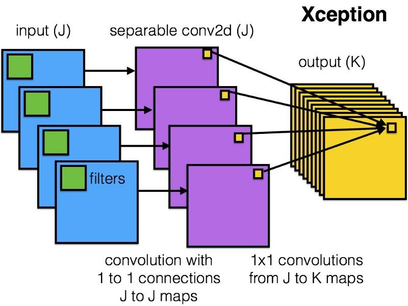
will like this network because of the simplicity and elegance of its architecture:

It contains 36 stages of folding, and this is similar to ResNet-34. At the same time, the model and code are simple, as in ResNet, and much more pleasant than in Inception V4.
A torch7 implementation of this network is available here , while a Keras / TF implementation is available here.
Curiously, the authors of the recent Xception architecture were also inspired by our work on separable convolutional filters .
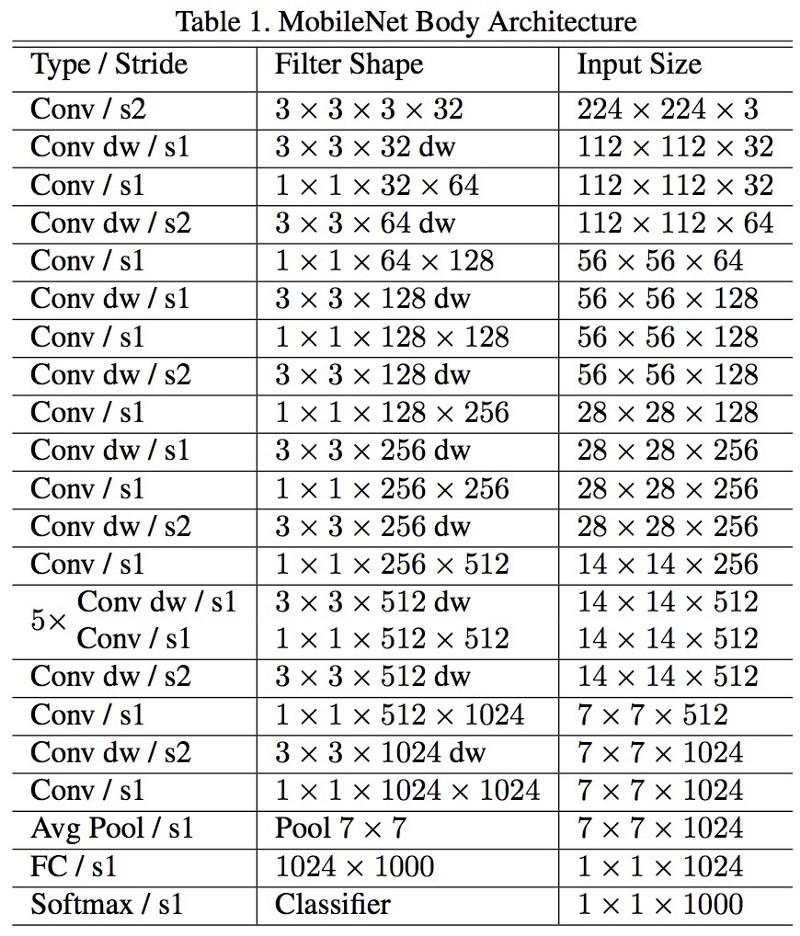
The new architecture of M obileNets was released in April 2017. To reduce the number of parameters, it uses detachable convolutions, the same as in Xception. It is also stated in the work that the authors were able to greatly reduce the number of parameters: about half in the case of FaceNet. Full architecture of the model:
We tested this network in a real task and found that it works incommensurably slowly on a package of 1 (batch of 1) on a Titan Xp graphics card. Compare the output duration for a single image:
This can not be called fast work! The number of parameters and the network size on the disk are reduced, but there is no sense in this.
FractalNet uses a recursive architecture that has not yet been tested on ImageNet and is a derivative or more general version of ResNet.
We believe that the development of neural network architectures is of paramount importance for the development of deep learning. We highly recommend that you carefully read and ponder all the work given here.
You may ask why we should spend so much time on the development of architectures, and why instead we do not use data that will tell us exactly what to use and how to combine the modules? A tempting opportunity, but work on it is still underway. Here are some initial results.
In addition, we talked only about architectures for computer vision. Other areas of development are also underway, and it would be interesting to study evolution in other areas.
If you are interested in comparing neural network performance and computing performance, seeour recent work .
Deep neural network algorithms have gained great popularity today, which is largely ensured by the well-thought-out architecture. Let's look at the history of their development over the past few years. If you are interested in a deeper analysis, refer to this work .
Comparison of popular architectures for Top-1 one-crop accuracy and the number of operations required for one direct pass. More details here .
Lenet5
In 1994, one of the first convolutional neural networks was developed, which laid the foundation for deep learning. This pioneering work by Yann LeCun, after many successful iterations since 1988, was called LeNet5 !
The LeNet5 architecture has become fundamental to deep learning, especially in terms of the distribution of image properties throughout the picture. Convolutions with learning parameters allowed using several parameters to efficiently extract the same properties from different places. In those years, there were no video cards that could speed up the learning process, and even the central processors were slow. Therefore, the key advantage of the architecture was the ability to save parameters and calculation results, in contrast to using each pixel as separate input data for a large multilayer neural network. In LeNet5, pixels are not used in the first layer, because images are strongly spatially correlated, so using individual pixels as input properties will not allow you to take advantage of these correlations.
Features of LeNet5:
- A convolutional neural network that uses a sequence of three layers: convolution layers, pooling layers and non-linearity layers -> since the publication of Lekun’s work, this is perhaps one of the main features of deep learning in relation to images.
- Uses convolution to retrieve spatial properties.
- Subsampling using spatial map averaging.
- Nonlinearity in the form of hyperbolic tangent or sigmoid.
- The final classifier in the form of a multilayer neural network (MLP).
- The sparse matrix of connectivity between the layers reduces the amount of computation.
This neural network formed the basis of many subsequent architectures and inspired many researchers.
Development
From 1998 to 2010, the neural networks were in a state of incubation. Most people did not notice their growing capabilities, although many developers gradually honed their algorithms. Thanks to the heyday of mobile phone cameras and the cheapening of digital cameras, more and more training data has become available to us. At the same time, computing capabilities grew, processors became more powerful, and video cards turned into the main computing tool. All these processes allowed the development of neural networks, albeit rather slowly. Interest in tasks that could be solved with the help of neural networks was growing, and finally the situation became obvious ...
Dan ciresan net
In 2010, Dan Claudiu Ciresan and Jurgen Schmidhuber published one of the first descriptions of the implementation of GPU neural networks . Their work contained the direct and reverse implementation of a 9-layer neural network on the NVIDIA GTX 280 .
Alexnet
In 2012, Alexei Krizhevsky published AlexNet , an in-depth and extended version of LeNet, which won by a wide margin in the ImageNet competition.
At AlexNet, the results of LeNet calculations are scaled into a much larger neural network, which is able to study much more complex objects and their hierarchies. Features of this solution:
- Use of linear rectification units (ReLU) as non-linearities.
- The use of discarding techniques for selective ignoring of individual neurons during training, which avoids over-training of the model.
- Overlap max pooling, which avoids the effects of averaging average pooling.
- Using NVIDIA GTX 580 to speed up learning.
By that time, the number of cores in video cards had grown significantly, which allowed them to reduce the training time by about 10 times, and as a result it became possible to use much larger datasets and pictures.
The success of AlexNet launched a small revolution, convolutional neural networks turned into a workhorse of deep learning - this term now means "large neural networks that can solve useful problems."
Overfeat
In December 2013, the NYU laboratory of Jan Lekun published a description of Overfeat , a variant of AlexNet. Also, the article described the trained bounding boxes, and subsequently many other works on this topic were published. We believe that it is better to learn how to segment objects, rather than using artificial bounding boxes.
Vgg
In VGG networks developed at Oxford, in each convolutional layer, for the first time, 3x3 filters were used, and even these layers were combined in a sequence of convolutions.
This contradicts the principles laid down in LeNet, according to which large convolutions were used to extract the same image properties. Instead of the 9x9 and 11x11 filters used in AlexNet, much smaller filters began to be used, dangerously close to 1x1 convolutions, which LeNet authors tried to avoid, at least in the first layers of the network. But the great advantage of VGG was the finding that several 3x3 convolutions combined in a sequence can emulate larger receptive fields, for example, 5x5 or 7x7. These ideas will later be used in the Inception and ResNet architectures.
VGG networks use multiple 3x3 convolutional layers to represent complex properties. Pay attention to blocks 3, 4 and 5 in VGG-E: to extract more complex properties and combine them, 256 × 256 and 512 × 512 3 × 3 filter sequences are used. This is equivalent to a large convolutional classifier 512x512 with three layers! This gives us a huge number of parameters and excellent learning abilities. But it was difficult to learn such networks; I had to break them into smaller ones, adding layers one by one. The reason was the lack of effective ways to regularize models or some methods of limiting a large search space, which is promoted by many parameters.
VGG in many layers use a large number of properties, so training was computationally expensive. The load can be reduced by reducing the number of properties, as is done in the bottleneck layers of the Inception architecture.
Network-in-network
The Network-in-network (NiN) architecture is based on a simple idea: using 1x1 convolutions to increase the combinatoriality of properties in convolutional layers.
In NiN, after each convolution, spatial MLP layers are used to better combine the properties before feeding to the next layer. It may seem that the use of 1x1 convolutions contradicts the original LeNet principles, but in reality it allows combining properties better than just stuffing more convolutional layers. This approach is different from using bare pixels as input for the next layer. In this case, 1x1 convolutions are used for spatial combination of properties after convolution within the framework of property maps, so you can use much fewer parameters that are common to all pixels of these properties!
MLP can greatly increase the effectiveness of individual convolutional layers by combining them into more complex groups. This idea was later used in other architectures, such as ResNet, Inception, and their variants.
GoogLeNet and Inception
Google Christian Szegedy is worried about lowering computations in deep neural networks, and as a result created GoogLeNet, the first Inception architecture .
By the fall of 2014, deep learning models had become very useful in categorizing image content and frames from videos. Many skeptics have recognized the benefits of deep learning and neural networks, and Internet giants, including Google, have become very interested in deploying efficient and large networks on their server capacities.
Christian was looking for ways to reduce the computational load in neural networks, achieving the highest performance (for example, in ImageNet). Or preserving the amount of computation, but still increasing productivity.
As a result, the command created an Inception module:
At first glance, this is a parallel combination of convolutional filters 1x1, 3x3 and 5x5. But the highlight was the use of convolution blocks 1x1 (NiN) to reduce the number of properties before serving in the "expensive" parallel blocks. Usually this part is called bottleneck, it is described in more detail in the next chapter.
GoogLeNet uses a stem without Inception modules as the initial layer, and also uses average pooling and a softmax classifier similar to NiN. This classifier performs extremely few operations compared to AlexNet and VGG. It also helped create a very efficient neural network architecture .
Bottleneck layer
This layer reduces the number of properties (and therefore operations) in each layer, so that the speed of obtaining the result can be maintained at a high level. Before transferring data to “expensive” convolutional modules, the number of properties is reduced, say, 4 times. This greatly reduces the amount of computation, which has made the architecture popular.
Let's figure it out. Suppose we have 256 properties at the input and 256 at the output, and let the Inception layer perform only 3x3 convolutions. We get 256x256x3x3 convolutions (589,000 operations of accumulation multiplication, that is, MAC operations). This may go beyond our computational speed requirements; let's say a layer is processed in 0.5 milliseconds on Google Server. Then reduce the number of properties for folding to 64 (256/4). In this case, we first perform a 1x1 convolution of 256 -> 64, then another 64 convolution in all Inception branches, and then again apply a 1x1 convolution of 64 -> 256 properties. Number of operations:
- 256 × 64 × 1 × 1 = 16,000
- 64 × 64 × 3 × 3 = 36,000
- 64 × 256 × 1 × 1 = 16,000
Only about 70,000, reduced the number of operations by almost 10 times! But at the same time, we did not lose generalization in this layer. Bottleneck layers have shown excellent performance on the ImageNet dataset, and have been used in later architectures such as ResNet. The reason for their success is that the input properties are correlated, which means that you can get rid of redundancy by correctly combining properties with 1x1 convolutions. And after folding with fewer properties, you can again deploy them into a significant combination on the next layer.
Inception V3 (and V2)
Christian and his team have proven to be very effective researchers. In February 2015, the Batch-normalized Inception architecture was introduced as the second version of Inception . Batch-normalization calculates the mean and standard deviation of all property distribution maps in the output layer, and normalizes their responses with these values. This corresponds to the "whitening" of the data, that is, the responses of all neural maps lie in the same range and with a zero mean. This approach makes learning easier, because the next layer is not required to remember offsets of input data and can only search for the best combinations of properties.
In December 2015, a new version of Inception modules and the corresponding architecture was released. The author’s article better explains the original GoogLeNet architecture, which tells much more about the decisions made. Key ideas:
- Maximizing the flow of information in the network due to the careful balance between its depth and width. Before each pooling, property maps increase.
- With increasing depth, the number of properties or layer width also systematically increases.
- The width of each layer increases to increase the combination of properties before the next layer.
- To the extent possible, only 3x3 convolutions are used. Given that the 5x5 and 7x7 filters can be decomposed using several 3x3, the
new Inception module looks like this: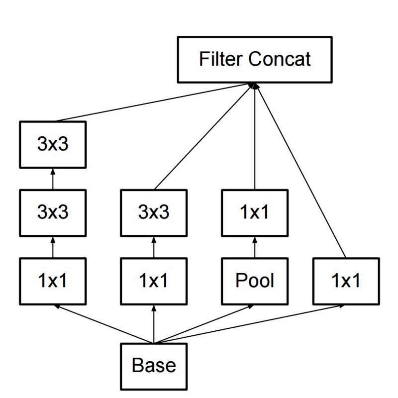
- Filters can also be decomposed using smoothed convolutions into more complex modules:

- Inception modules can reduce the size of data using pooling during Inception calculations. This is similar to performing convolution with strides in parallel with a simple pooling layer:

Inception uses the pooling layer with softmax as the final classifier.
Resnet
In December 2015, at about the same time that the Inception v3 architecture was introduced, a revolution occurred - they published ResNet . It contains simple ideas: submit the output of two successful convolutional layers And bypass the input for the next layer!
Such ideas have already been proposed, for example, here . But in this case, the authors bypass TWO layers and apply the approach on a large scale. Bypassing one layer does not give much benefit, and bypassing two is a key find. This can be seen as a small classifier, as network-in-network!
It was also the first ever example of training a network of several hundred, even thousands of layers.
Multilayer ResNet used a bottleneck layer similar to that used in Inception:
This layer reduces the number of properties in each layer, first using a 1x1 convolution with a smaller output (usually a quarter of the input), then a 3x3 layer, and then again convolving 1x1 into a larger number of properties. As in the case of Inception modules, this saves computational resources while maintaining a wealth of property combinations. Compare with the more complex and less obvious stems in Inception V3 and V4.
ResNet uses a pooling layer with softmax as the final classifier.
Every day, additional information about the ResNet architecture appears:
- It can be considered as a system of simultaneously parallel and serial modules: in many modules the inout-signal comes in parallel, and the output signals of each module are connected in series.
- ResNet can be considered as several ensembles of parallel or serial modules .
- It turned out that ResNet usually operates with relatively small depth blocks of 20-30 layers working in parallel, rather than running sequentially along the entire length of the network.
- Since the output signal comes back and is fed as an input, as is done in RNN, ResNet can be considered an improved plausible model of the cerebral cortex .
Inception V4
Christian and his team excelled again with a new version of Inception .
The Inception-module that comes after stem is the same as in Inception V3:
In this case, the Inception-module is combined with the ResNet-module:
This architecture turned out, to my taste, more complicated, less elegant, and also filled with opaque heuristic solutions. It is difficult to understand why the authors made these or those decisions, and it is equally difficult to give them any kind of assessment.
Therefore, the prize for a clean and simple neural network, easy to understand and modify, goes to ResNet.
Squeezenet
SqueezeNet published recently. This is a remake in a new way of many concepts from ResNet and Inception. The authors demonstrated that improving the architecture reduces network size and the number of parameters without complex compression algorithms.
ENet
All the features of recent architectures are combined into a very efficient and compact network, using very few parameters and computing power, but at the same time giving excellent results. The architecture was called ENet , it was developed by Adam Paszke ( Adam Paszke ). For example, we used it for very accurate marking of objects on the screen and parsing scenes. A few examples of Enet . These videos are not related to the training dataset .
HereYou can find the technical details of ENet. It is a network based on encoder and decoder. The encoder is built on the usual CNN categorization scheme, and the decoder is an upsampling netowrk designed for segmentation by spreading the categories back to the original size image. For image segmentation, only neural networks were used, no other algorithms.
As you can see, ENet has the highest specific accuracy compared to all other neural networks.
ENet was designed to use as few resources as possible from the very beginning. As a result, the encoder and decoder together occupy only 0.7 MB with fp16 precision. And with such a tiny size, ENet is not inferior to segmentation accuracy or superior to other purely neural network solutions.
Module analysis
Published a systematic assessment of CNN modules. It turned out to be beneficial:
- Use ELU non-linearity without batch normalization (batchnorm) or ReLU with normalization.
- Apply learned transformation of RGB color space.
- Use a linear learning rate decay policy.
- Use the sum of the middle and maximum pooling layer.
- Use a 128 or 256 mini-packet. If this is too much for your video card, reduce the learning speed in proportion to the packet size.
- Use fully connected layers as convolutional layers and average forecasts to give the final solution.
- If you increase the size of the training dataset, make sure that you have not reached a plateau in training. Data cleanliness is more important than size.
- If you can’t increase the size of the input image, reduce the stride in subsequent layers, the effect will be approximately the same.
- If your network has a complex and highly optimized architecture, as in GoogLeNet, then modify it with caution.
Xception
Xception introduced a simpler and more elegant architecture into the Inception module, which is no less efficient than ResNet and Inception V4.
Here's what the Xception module looks like: Anyone
will like this network because of the simplicity and elegance of its architecture:
It contains 36 stages of folding, and this is similar to ResNet-34. At the same time, the model and code are simple, as in ResNet, and much more pleasant than in Inception V4.
A torch7 implementation of this network is available here , while a Keras / TF implementation is available here.
Curiously, the authors of the recent Xception architecture were also inspired by our work on separable convolutional filters .
MobileNets
The new architecture of M obileNets was released in April 2017. To reduce the number of parameters, it uses detachable convolutions, the same as in Xception. It is also stated in the work that the authors were able to greatly reduce the number of parameters: about half in the case of FaceNet. Full architecture of the model:
We tested this network in a real task and found that it works incommensurably slowly on a package of 1 (batch of 1) on a Titan Xp graphics card. Compare the output duration for a single image:
- resnet18: 0.002871
- alexnet: 0.001003
- vgg16: 0.001698
- squeezenet: 0.002725
- mobilenet: 0.033251
This can not be called fast work! The number of parameters and the network size on the disk are reduced, but there is no sense in this.
Other notable architectures
FractalNet uses a recursive architecture that has not yet been tested on ImageNet and is a derivative or more general version of ResNet.
Future
We believe that the development of neural network architectures is of paramount importance for the development of deep learning. We highly recommend that you carefully read and ponder all the work given here.
You may ask why we should spend so much time on the development of architectures, and why instead we do not use data that will tell us exactly what to use and how to combine the modules? A tempting opportunity, but work on it is still underway. Here are some initial results.
In addition, we talked only about architectures for computer vision. Other areas of development are also underway, and it would be interesting to study evolution in other areas.
If you are interested in comparing neural network performance and computing performance, seeour recent work .