The incredible adventures of Robert Hanbury Brown and Richard Twiss. Part 3: from telescope to quantum computing
Ending. Start here: part 1 , part 2 .
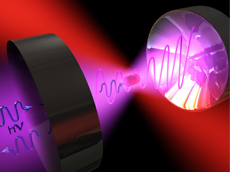
In English, rocket science is said about complex and obscure things. In Russian, they often resort to comparison with the theory of relativity or quantum mechanics. Although the latter begins with very simple ideas: let's say that light is propagated by individual particles - photons. In a second you can see 96, 97 or 99 photons, and never - 99 and a half. This surprisingly simple idea leads to very unusual consequences.
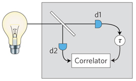
Before pointing a double telescope at SiriusOur heroes decided to test it in the laboratory. The star was played by the light of a lamp focused on a small hole, and instead of two telescopes, two photomultipliers were used. It was not possible to place them side by side, so they came up with a trick: the light from the “star” was sent to a translucent mirror, which reflected one half of the radiation and the other transmitted. One photomultiplier looked at the reflection of the "star", the second stood behind the mirror and saw the "star" in the light:
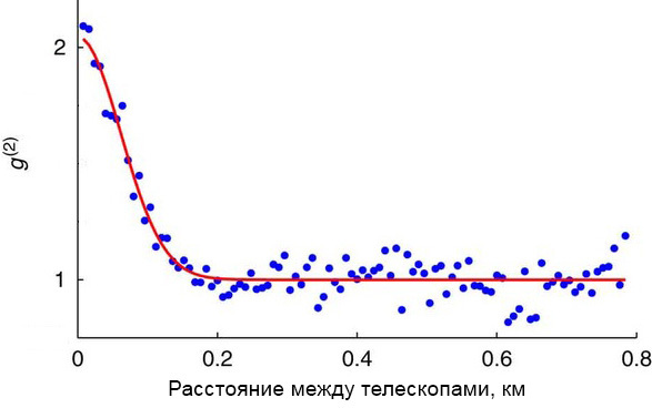
The experiment showed that Twiss's theory is correct: the more “apart” the photomultipliers, the smaller the measured correlation. But here an interesting question arose. A photomultiplier is a very sensitive photodetector, its main task is to generate a powerful current pulse for one incoming photon:
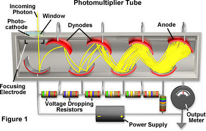
Photomultiplier. A photon flew from the top left and generated an electron. It was accelerated by a field, hit a dynode (intermediate anode) and knocked out two electrons from it. These two electrons also accelerated and knocked four electrons out of the next dynode, and so on. As a result, a single photon generated such a good current pulse.
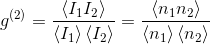
The photomultiplier sees not light, but single photons. This is logical: after all, the intensity of light is simply the number of photons arriving in a second. But then the correlation should be considered not for a noisy signal, but for photons. Reasonable, why not? Just replace the intensity ( I ) with the number of photons ( n ):
For independent sources, the correlation is one. Logically: this is the case of divorced telescopes when they see different parts of a star. But when the telescopes are “shifted”, the correlation becomes equal to two. This means that photons do not come independently, but in pairs! How so?
The time has come to recall the fundamental property of quantum optics: an integer number of photons always comes for any time interval. Based on this property, Roy Glauber of Harvard creates a coherence theory that describes the properties of photons, their statistics, coherence, and all that. It is based on the second quantization method, which uses the creation and annihilation operators of photons - the names speak for themselves: photons appear and disappear individually, and their total number always remains intact.
Glauber's coherence theory described in detail the Hanbury Brown – Twiss experiment and showed that photons from a star (and from any other heat source — lamps, LEDs, gas discharges, etc.) really “try” to come in pairs. The same theory explained the physical meaning of this mysterious correlation function g (2) : it shows how “friendly” the source emits photons. If g (2) is greater than unity, then photons prefer to radiate in groups; if less than one, then separately. Well, g (2) = 1 corresponds to photons that are emitted independently. Oddly enough, the laser also generates light with g (2) = 1.
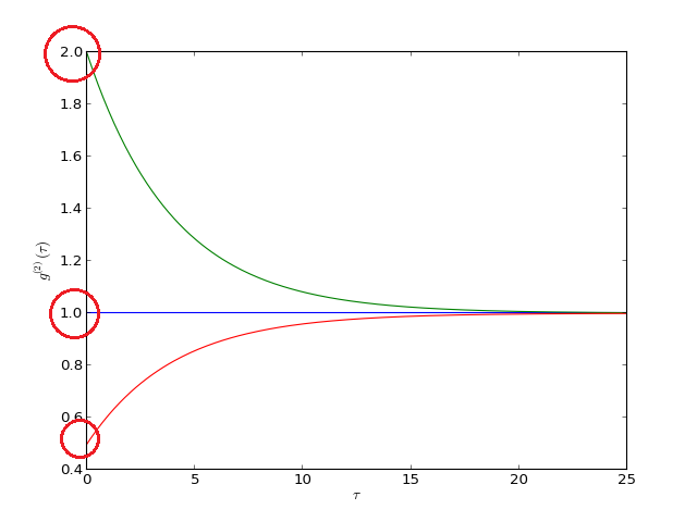 In circles there are different g (2) values for “shifted” telescopes. For "spread" g (2) is always equal to unity (right).
As expected, g (2) = 2 means that photons come in pairs, and the experiment is correct. The Hanbury Brown family celebrated this joyful event with the birth of two twins.
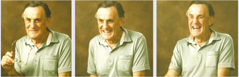
Robert Hanbury Brown is definitely pleased with what is happening.
I talked about the theory of coherence and about the magic of double photons, but it turned out somehow incomprehensibly. Fortunately, the theory has a more visual description. If the source emits an average of 22.5 photons per second, then every second we will most likely detect 22 or 23 photons, less often 15 or 30, and almost never zero or one hundred. The distribution of the number of photons with a maximum at 22.5 looms:
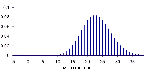
And how wide is it? It turns out that for "good" radiation (if the photons are emitted independently of each other) centered on N, the distribution width is equal to the root of N. This distribution is called Poisson . If the distribution turns out to be wider, it is called Super Poisson (and the narrower - sub Poisson ):
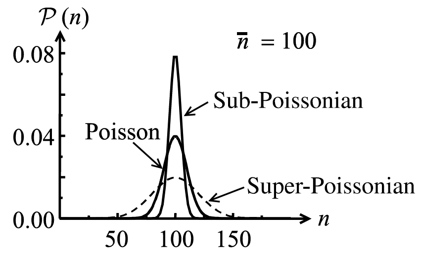
Poisson, sub-Poisson and super-Poisson statistics.
Well, the function g (2) shows the width of the distribution: the larger it is, the wider the distribution. g (2) = 1 corresponds to the Poisson distribution, while it does not depend on the average number of photons. That is, for any laser - both for the weak and for the powerful - g (2) is equal to unity.
For thermal light, g (2) = 2. Does this mean that the distribution is twice as wide as the laser? Not really. It is wider than the laser, but it looks completely different:
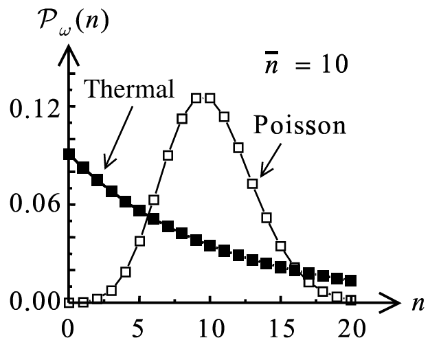
That is, thermal radiation is somewhat similar to the distribution of energy levels: the higher the level (the greater the number of photons), the less likely it is to see it. Hence the main conclusion: thermal and coherent radiation have fundamentally different statistical properties . The best part is that measuring g (2) with the Hanbury Brown-Twiss experiment allows us to easily measure these statistics. Where does this apply? Well, for example, in the development of lasers: using g (2), one can determine the generation threshold (that is, the conditions under which radiation from thermal becomes laser).
Well, the most interesting (and useful) case is g (2)= 0. The width of the photon distribution is zero! What does it mean? It turns out that the number of photons is strictly fixed and does not change from second to second. The distribution consists of a single peak (right picture):

Photon statistics: Poisson (it is also coherent, g (2) = 1), thermal (g (2) = 2), Fokowska (it is also N-photon, g (2) = 0).
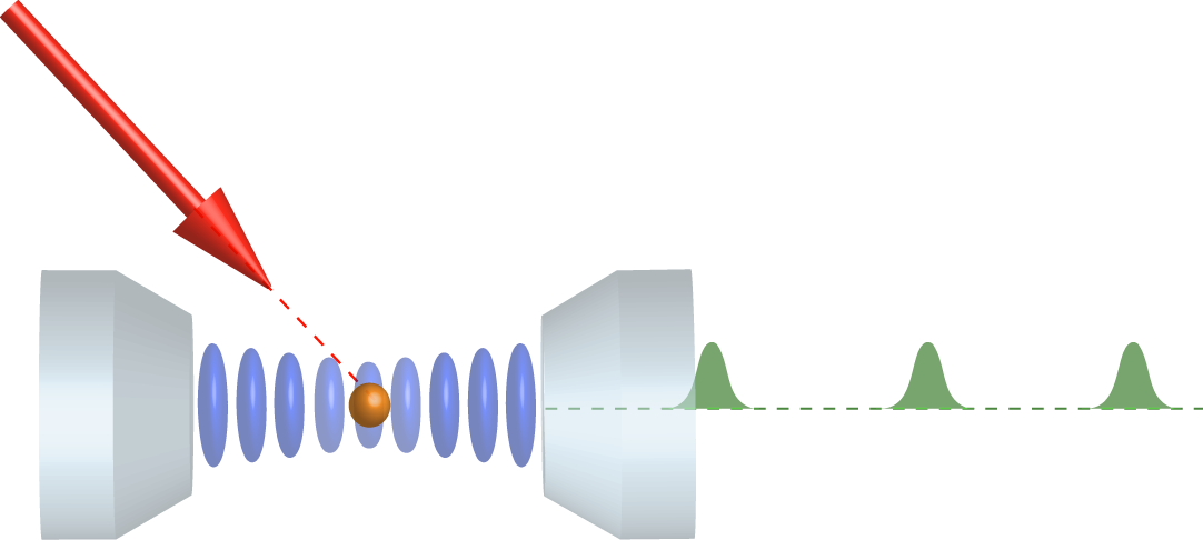
The most interesting thing happens when the source emits exactly one photon (the cap suggests that such a thing is called a single-photon source) Such devices are needed for the operation of optical transistors, switching qubits, in quantum cryptography and similar applications. The requirements for them are very serious: they should in no case generate more than one photon. Otherwise, a randomly emitted photon can lead to information leakage. Or, for example, the optical key will turn on from the first photon and immediately turn off from the second. Therefore, single-photon sources must be thoroughly tested.
How to detect one photon (or better, two)? A conventional photodiode is useless: the response will be too weak. They use an avalanche diode - but it has its drawbacks. For example, it has dead time : for each photon that arrives, it generates a long current pulse, and the second photon arrives at this time, the diode simply does not notice it:
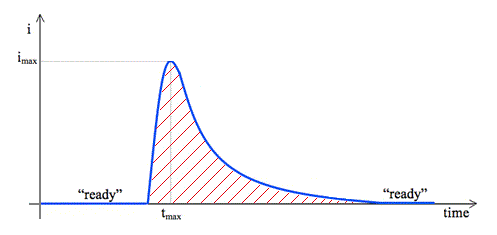
Red hatching is dead time. Usually it is not less than 100 picoseconds.
The idea of our main characters comes to the rescue: let's direct the light to a translucent mirror and two detectors, and then calculate the value of g (2) . If g (2) = 0, then the source is single-photon, if g (2) > 0, then sometimes it emits two photons. And now - attention, physical magic! - three explanations of why this works:
1. From a picture with distributions.

If every second the source emits one photon, then the histogram has one column at “1”, the distribution width is zero and g (2) = 0. If 2 photons are sometimes emitted, then the column at “2” appears in the histogram and the distribution width grows, and g (2) also grows with it .
2. From the formula
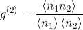
If the source is single-photon, then n1 + n2 = 1, which means that one of the numbers is zero, which means that the product of n1 and n2 is also zero, as well as g (2) . If two photons are emitted (n1 + n2 = 2), then maybe n1 = n2 = n1 * n2 = 1, and g (2) becomes greater than zero.
3. And, finally, the most important thing: from common sense! If photons are emitted in pairs, then from time to time one photon will hit one diode, and the second to the second. Then we will see synchronous triggering of the diodes - coincidences that increase the value of g (2) . If the source is truly single-photon, then the diodes will never operate simultaneously.
Hanbury Brown-Twiss idea is completely indispensable in the analysis of single-photon sources. For a good source, the correlation function g (2) looks something like this:

Here the zero is not in the left, but in the middle; to the left are the negative shifts of one of the detectors (as if the left telescope was to the right than the right). The main thing is invariable: at zero time delay g (2) reaches zero, at a very large delay photons are emitted independently and g (2) = 1.
But a not-so-good source looks something like this:
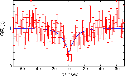
It can be seen that the function does not fall below 0.4. This means that the source often emits pairs of photons, and for especially important applications it is better to look for another one.
Roy Glauber received the Nobel Prize for the theory of coherence in 2005. Our main characters could not share it: Richard Twiss did not live up to this moment only six months; three years earlier Robert Hanbury Brown was gone. But, as you know, the greatest recognition is when your name becomes a household name. A simple and brilliant idea - measuring correlations using a glass plate and two diodes - remained in history under the name Hanbury Brown-Twiss circuit .

Pictures from 2015 articles in the top scientific journals Nature and Science with measurement of correlations using the Hanbury Brown-Twiss scheme. The task of observation: find it in five places :).
This ends the story, but its logical continuation can be found here.
Sources of
M. Fox. Quantum optics: An Introduction - Oxford University Press, 2006.
R. Hanbury Brown. The Intensity Interferometer. Its Application to Astronomy. - London: Taylor & Francis, 1974.
R. Hanbury Brown. Boffin: A Personal Story of the Early Days of Radar, Radio Astronomy and Quantum Optics - Bristol: Adam Hilger, 1991.
Obituary: Robert Hanbury Brown. Nature 416, 34 (2002).
Pictures: 1 , 2 , 3 , 4 , 5 , 6 , 7 , 8 , 9 , 10 , 11 .
In English, rocket science is said about complex and obscure things. In Russian, they often resort to comparison with the theory of relativity or quantum mechanics. Although the latter begins with very simple ideas: let's say that light is propagated by individual particles - photons. In a second you can see 96, 97 or 99 photons, and never - 99 and a half. This surprisingly simple idea leads to very unusual consequences.
Before pointing a double telescope at SiriusOur heroes decided to test it in the laboratory. The star was played by the light of a lamp focused on a small hole, and instead of two telescopes, two photomultipliers were used. It was not possible to place them side by side, so they came up with a trick: the light from the “star” was sent to a translucent mirror, which reflected one half of the radiation and the other transmitted. One photomultiplier looked at the reflection of the "star", the second stood behind the mirror and saw the "star" in the light:
The experiment showed that Twiss's theory is correct: the more “apart” the photomultipliers, the smaller the measured correlation. But here an interesting question arose. A photomultiplier is a very sensitive photodetector, its main task is to generate a powerful current pulse for one incoming photon:
Photomultiplier. A photon flew from the top left and generated an electron. It was accelerated by a field, hit a dynode (intermediate anode) and knocked out two electrons from it. These two electrons also accelerated and knocked four electrons out of the next dynode, and so on. As a result, a single photon generated such a good current pulse.
The photomultiplier sees not light, but single photons. This is logical: after all, the intensity of light is simply the number of photons arriving in a second. But then the correlation should be considered not for a noisy signal, but for photons. Reasonable, why not? Just replace the intensity ( I ) with the number of photons ( n ):
For independent sources, the correlation is one. Logically: this is the case of divorced telescopes when they see different parts of a star. But when the telescopes are “shifted”, the correlation becomes equal to two. This means that photons do not come independently, but in pairs! How so?
The time has come to recall the fundamental property of quantum optics: an integer number of photons always comes for any time interval. Based on this property, Roy Glauber of Harvard creates a coherence theory that describes the properties of photons, their statistics, coherence, and all that. It is based on the second quantization method, which uses the creation and annihilation operators of photons - the names speak for themselves: photons appear and disappear individually, and their total number always remains intact.
Glauber's coherence theory described in detail the Hanbury Brown – Twiss experiment and showed that photons from a star (and from any other heat source — lamps, LEDs, gas discharges, etc.) really “try” to come in pairs. The same theory explained the physical meaning of this mysterious correlation function g (2) : it shows how “friendly” the source emits photons. If g (2) is greater than unity, then photons prefer to radiate in groups; if less than one, then separately. Well, g (2) = 1 corresponds to photons that are emitted independently. Oddly enough, the laser also generates light with g (2) = 1.
As expected, g (2) = 2 means that photons come in pairs, and the experiment is correct. The Hanbury Brown family celebrated this joyful event with the birth of two twins.
Robert Hanbury Brown is definitely pleased with what is happening.
I talked about the theory of coherence and about the magic of double photons, but it turned out somehow incomprehensibly. Fortunately, the theory has a more visual description. If the source emits an average of 22.5 photons per second, then every second we will most likely detect 22 or 23 photons, less often 15 or 30, and almost never zero or one hundred. The distribution of the number of photons with a maximum at 22.5 looms:
And how wide is it? It turns out that for "good" radiation (if the photons are emitted independently of each other) centered on N, the distribution width is equal to the root of N. This distribution is called Poisson . If the distribution turns out to be wider, it is called Super Poisson (and the narrower - sub Poisson ):
Poisson, sub-Poisson and super-Poisson statistics.
Well, the function g (2) shows the width of the distribution: the larger it is, the wider the distribution. g (2) = 1 corresponds to the Poisson distribution, while it does not depend on the average number of photons. That is, for any laser - both for the weak and for the powerful - g (2) is equal to unity.
For thermal light, g (2) = 2. Does this mean that the distribution is twice as wide as the laser? Not really. It is wider than the laser, but it looks completely different:
That is, thermal radiation is somewhat similar to the distribution of energy levels: the higher the level (the greater the number of photons), the less likely it is to see it. Hence the main conclusion: thermal and coherent radiation have fundamentally different statistical properties . The best part is that measuring g (2) with the Hanbury Brown-Twiss experiment allows us to easily measure these statistics. Where does this apply? Well, for example, in the development of lasers: using g (2), one can determine the generation threshold (that is, the conditions under which radiation from thermal becomes laser).
Well, the most interesting (and useful) case is g (2)= 0. The width of the photon distribution is zero! What does it mean? It turns out that the number of photons is strictly fixed and does not change from second to second. The distribution consists of a single peak (right picture):
Photon statistics: Poisson (it is also coherent, g (2) = 1), thermal (g (2) = 2), Fokowska (it is also N-photon, g (2) = 0).
The most interesting thing happens when the source emits exactly one photon (the cap suggests that such a thing is called a single-photon source) Such devices are needed for the operation of optical transistors, switching qubits, in quantum cryptography and similar applications. The requirements for them are very serious: they should in no case generate more than one photon. Otherwise, a randomly emitted photon can lead to information leakage. Or, for example, the optical key will turn on from the first photon and immediately turn off from the second. Therefore, single-photon sources must be thoroughly tested.
How to detect one photon (or better, two)? A conventional photodiode is useless: the response will be too weak. They use an avalanche diode - but it has its drawbacks. For example, it has dead time : for each photon that arrives, it generates a long current pulse, and the second photon arrives at this time, the diode simply does not notice it:
Red hatching is dead time. Usually it is not less than 100 picoseconds.
The idea of our main characters comes to the rescue: let's direct the light to a translucent mirror and two detectors, and then calculate the value of g (2) . If g (2) = 0, then the source is single-photon, if g (2) > 0, then sometimes it emits two photons. And now - attention, physical magic! - three explanations of why this works:
1. From a picture with distributions.
If every second the source emits one photon, then the histogram has one column at “1”, the distribution width is zero and g (2) = 0. If 2 photons are sometimes emitted, then the column at “2” appears in the histogram and the distribution width grows, and g (2) also grows with it .
2. From the formula
If the source is single-photon, then n1 + n2 = 1, which means that one of the numbers is zero, which means that the product of n1 and n2 is also zero, as well as g (2) . If two photons are emitted (n1 + n2 = 2), then maybe n1 = n2 = n1 * n2 = 1, and g (2) becomes greater than zero.
3. And, finally, the most important thing: from common sense! If photons are emitted in pairs, then from time to time one photon will hit one diode, and the second to the second. Then we will see synchronous triggering of the diodes - coincidences that increase the value of g (2) . If the source is truly single-photon, then the diodes will never operate simultaneously.
Hanbury Brown-Twiss idea is completely indispensable in the analysis of single-photon sources. For a good source, the correlation function g (2) looks something like this:
Here the zero is not in the left, but in the middle; to the left are the negative shifts of one of the detectors (as if the left telescope was to the right than the right). The main thing is invariable: at zero time delay g (2) reaches zero, at a very large delay photons are emitted independently and g (2) = 1.
But a not-so-good source looks something like this:
It can be seen that the function does not fall below 0.4. This means that the source often emits pairs of photons, and for especially important applications it is better to look for another one.
Roy Glauber received the Nobel Prize for the theory of coherence in 2005. Our main characters could not share it: Richard Twiss did not live up to this moment only six months; three years earlier Robert Hanbury Brown was gone. But, as you know, the greatest recognition is when your name becomes a household name. A simple and brilliant idea - measuring correlations using a glass plate and two diodes - remained in history under the name Hanbury Brown-Twiss circuit .
Pictures from 2015 articles in the top scientific journals Nature and Science with measurement of correlations using the Hanbury Brown-Twiss scheme. The task of observation: find it in five places :).
This ends the story, but its logical continuation can be found here.
Sources of
M. Fox. Quantum optics: An Introduction - Oxford University Press, 2006.
R. Hanbury Brown. The Intensity Interferometer. Its Application to Astronomy. - London: Taylor & Francis, 1974.
R. Hanbury Brown. Boffin: A Personal Story of the Early Days of Radar, Radio Astronomy and Quantum Optics - Bristol: Adam Hilger, 1991.
Obituary: Robert Hanbury Brown. Nature 416, 34 (2002).
Pictures: 1 , 2 , 3 , 4 , 5 , 6 , 7 , 8 , 9 , 10 , 11 .