Walk between pixels
- Transfer
This post relates to my article on calculating points on Bezier curves using linear texture interpolation. The extended method extends to Bezier surfaces and (multidimensional) polynomials.
The initial observation was that if you sample on a 2 × 2 texture diagonal, then the output will be points on the quadratic Bezier curve, and the reference points on the curve are pixel values, as in the image below. When I say that you get a quadratic Bezier curve, I express myself literally and accurately. This can be represented as follows: texture interpolation literally executes the de Casteljo algorithm. (Note: if the “B” values are not equal in the example below, then the second reference point will be the middle of these two values: the extension will abuse it to approximate more curves to fewer pixels).

My plans have long been to see what happens when sampling pixels in other directions than the 45 ° diagonal. In particular, the following are of interest:
When I accidentally stumbled upon the answer to the first question, it was time to look at the others!
P. S. What is the use of this? The best thing that comes to mind is data compression on the GPU. If approximated by piecewise rational polynomials, then the ideas of this method are useful for compressing data (pixels in a texture) that are quickly and easily decoded by the GPU. The ideas from this article allow us to use other types of curves for approximating and storing data, except for piecewise rational polynomials. In addition, curves and higher-order surfaces take up less texture.
Bilinear interpolation is available on modern GPUs as a way to obtain subpixel detail. In the old days, when scaling a texture, square pixels simply increased because interpolation was used for the nearest neighboring points. Nowadays, bilinear interpolation fills the space between pixels better than interpolation at the nearest neighboring points.
Bilinear interpolation can be described as interpolating two values along the x axis and interpolating the results along the y axis (or in reverse). Mathematically, it looks like this:
Where x and y are values from 0 to 1 that describe the location of the point between the pixels, and A, B, C and D are the values of the four nearest pixels that form a rectangle around the point we are calculating. A = (0,0), B = (1,0), C = (0,1) and D = (1,1).
After some transformations, this equation is presented in the form of a power series, which is better suited for our experiments:
For more information on bilinear interpolation, study these materials: 1 , 2 , 3 , 4 .
With the formula on hand you can start!
So, we know that if the sample goes diagonally from A to D, then we get a quadratic equation. What will happen on other lines?
Before I knew the answer, I assumed that if a line at an angle of 45 ° gives a quadratic equation (degree 2), and horizontal and vertical lines give a linear equation (degree 1), then the sample along other lines should be a polynomial with a degree between 1 and 2 The answer turned out to be different, but I was interested in whether it is possible to interpret the “real answer” in the form of a polynomial with degree between 1 and 2?
In any case, Wikipedia prompted me :
This means that the horizontal or vertical line will be a linear equation. Any other line gives a quadratic.
Let's check.
Remember that the equation for a linear function so literally replace
  on the
  and see what happens.
So, we start with the power series of the polynomial of bilinear interpolation:
After the replacement, it turns out:
After some expansion and simplification, we get the following:
This formula reports the value of the bilinear interpolation A, B, C and D (that is, the bilinear surface bounded by these points), and we sample along the x, y line defined by.
This is a very generalized function, which is difficult to talk about a lot, but one thing is clear: it is a quadratic function! Whatever constant values you choose for A, B, C, D, m, and b, you get a quadratic polynomial (or a lower degree, but never higher).
This shader shows the curves generated by random subpixel line segments on a random RGB texture (white noise).
(Note that the uneven edges of the curve are due to the fact that the interpolation takes place in the fixed-point format X.8, so the accuracy is quite limited. See the above scientific work for more information and ways to solve this problem).

Let's go ahead, indicate some values for and
and  and see what happens for different types of lines.
m = 0, b = 0
What happens if m and b are 0. In other words, what happens when sampling along the line .
.
Substitution of these values gives:
Interestingly, this is just linear interpolation between A and B, which makes sense when looking at a graph with a sample on a bilinear surface.
This is consistent with what Wikipedia told us: when one of the coordinates is unchanged (horizontal or vertical line), the result is linear.
m = 1, b = 0
Let's try m = 1 and b = 0. This is the line . The graph shows where the sample comes from on a bilinear surface:
Substitution of these values gives the following equation:
We got a quadratic equation, which should not be too surprising. It is also a formula for a quadratic Bezier curve with control points ,
,  ,
,  .
.
m = 2, b = 1
Let's try the line Here is the graph where we sample on a bilinear surface:
Substitution of values gives us the equation:
Again, a quadratic function is obtained.
You may be surprised that the equation ends instead
  but if you look at the chart, it makes sense. The line literally starts at point C when x is zero.
x = 2u, y = 3u
In the above examples, we change only the variable y as a function of x. What if we also change the variable x?
One option is to enter a third variable , which takes values from 0 to 1. Then we can express x and y through this variable.
Let's see what happens if you use these two equations:
The sample runs along such a line on a bilinear surface.

Substitution of the functions u for x and y gives:
This is still a quadratic equation!
So, now we know that when moving in a straight line on a bilinear surface, a quadratic function is obtained, except when the line is horizontal or vertical. Note: if a bilinear surface is a plane, then all the lines on this surface will be linear functions, so this is another way to get a linear result. It can also degenerate to a point. You will never get a cubic result (or higher) when moving in a straight line.
What happens if, instead of selecting along straight lines, other shapes, such as quadratic curves, are selected?
y = x * x
Let's start with the function . Here is the curve obtained:
Returning to the form of bilinear interpolation in the form of a power series, let's substitute instead and see what happens.
The initial equation is:
becomes like this:
It turns:
This is a cubic equation!
Here is a shader that draws this trajectory for random pixels: The

certain elegance of this example is that the cubic equation has four coefficients, which are based on four reference points, so that “everything goes into business,” so to speak.
This is not like sampling along linear segments where three anchor points are stored in four pixel values. One of them in this case is a little redundant.
You can use this fact, but sampling along a quadratic path to obtain a cubic curve seems like a natural approximation.
x = u * u, y = u * u
Let's see what happens if we move along x and y quadratically.
As in the linear case, we have our third variable u, which varies from 0 to 1, and we have x and y based on this variable. We will use the following equations:
The sampling path is as follows:
When we substitute the values, we obtain an equation of the fourth degree:
You may be surprised to see a linear path. It's just that x is always equal to y, even if they change non-linearly in the graph: a shader .
Let's frolic a little by taking these equations:
What corresponds to such a sampling path:
If you substitute the values, then the bilinear interpolation equation ...
... turns into an equation of the sixth degree:
The Shadertoy shader generator renders it at random pixels as usual, but if u changes from 0 to 1, then x changes from 0 to 3 (y is still in the range from 0 to 1), which leads to some obvious gaps at the borders of the pixels. In a purely mathematical formulation, there wouldn’t be anything like this, but we sample on a real texture, so when we leave our safe house (0,1), we find ourselves in a completely new territory with other reference points .

Let's try a function that follows a trajectory on a bilinear surface:
The bilinear interpolation equation becomes a trigonometric polynomial:
There are gaps due to going beyond the original pixel area, so in this case, this shader generated for . It scales and shifts the y values so that they are between 0 and 1.

Finally, circular sampling.
Here is its trajectory:
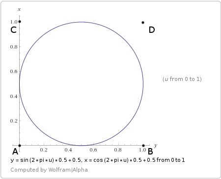
We substitute into the bilinear equation:
Matching Shaders .

A remarkable feature of the sample in a circle is its continuity. Notice how the left side of the curve quietly goes to the right. This seems like a pretty useful feature.
We went a bit into the wilds, but I hope you saw many opportunities for encoding and decoding data in a very small number of pixels, if you carefully select the selection path.
This is more complicated than the simple diagonal sampling method, and shader instructions are required. In particular, in the shader, you need to encode any change in x or y before transferring linear textures to the interpolator. This means that the method requires more ALU resources. But he saves texture memory.
The last question from those listed at the beginning of the article: how will sample patterns change in higher dimensions, such as trilinear or quadrilinear interpolation?
Well, here the mechanism is about the same as in bilinear interpolation, only more measurements.
In two-dimensional bilinear interpolation, we saw that after the transformation of x and y into functions (either from each other or from the third variable u), the resulting polynomial had a degree equal to the sum of the powers of x and y.
In three dimensions with trilinear interpolation, the resulting polynomial will have a degree equal to the sum of the degrees x, y, and z.
In four dimensions with quadrilinear interpolation, add another degree z.
Consider the case when we need not a curve, but a surface or (hyper) volume.
As we saw in an extension that works with surfaces and volumes, if we have a polynomial of degree N, then it can be divided into a multidimensional polynomial (also known as a surface or hypervolume), if the sum of the degrees of each axis is added to N.
This is something about we just talked, just the opposite.
There is something that I find interesting to study in the future - to see what limitations arise if one goes too far.
For example, a 2 × 2 texture can give a quadratic function if you sample along any line in the uv coordinates. If you first express the coordinate u in terms of a cubic function, and the coordinate v in terms of another cubic function, then I think that we can make a bicubic surface.
The surface will be limited to a subset of the possible shapes of the common bicubic surface, but you will actually get a bicubic surface (there will be mostly implicit anchor points that you do not control unless you add more pixels and make additional sampling or linear interpolation of a higher dimension).
I would like to see what restrictions there are and whether there is a chance to get real benefits from something like that.
Anyway, thanks for reading! Any ideas, corrections, use cases - throw me!
@ Atrix256
The initial observation was that if you sample on a 2 × 2 texture diagonal, then the output will be points on the quadratic Bezier curve, and the reference points on the curve are pixel values, as in the image below. When I say that you get a quadratic Bezier curve, I express myself literally and accurately. This can be represented as follows: texture interpolation literally executes the de Casteljo algorithm. (Note: if the “B” values are not equal in the example below, then the second reference point will be the middle of these two values: the extension will abuse it to approximate more curves to fewer pixels).
My plans have long been to see what happens when sampling pixels in other directions than the 45 ° diagonal. In particular, the following are of interest:
- What if you try a different line?
- What if you sample along a quadratic curve, for example, ?
- What if you try a circle or a sinusoid?
- How will sample patterns change in higher dimensions, like trilinear or quadrilinear interpolation?
When I accidentally stumbled upon the answer to the first question, it was time to look at the others!
P. S. What is the use of this? The best thing that comes to mind is data compression on the GPU. If approximated by piecewise rational polynomials, then the ideas of this method are useful for compressing data (pixels in a texture) that are quickly and easily decoded by the GPU. The ideas from this article allow us to use other types of curves for approximating and storing data, except for piecewise rational polynomials. In addition, curves and higher-order surfaces take up less texture.
Quick setup: bilinear interpolation formula
Bilinear interpolation is available on modern GPUs as a way to obtain subpixel detail. In the old days, when scaling a texture, square pixels simply increased because interpolation was used for the nearest neighboring points. Nowadays, bilinear interpolation fills the space between pixels better than interpolation at the nearest neighboring points.
Bilinear interpolation can be described as interpolating two values along the x axis and interpolating the results along the y axis (or in reverse). Mathematically, it looks like this:

Where x and y are values from 0 to 1 that describe the location of the point between the pixels, and A, B, C and D are the values of the four nearest pixels that form a rectangle around the point we are calculating. A = (0,0), B = (1,0), C = (0,1) and D = (1,1).
After some transformations, this equation is presented in the form of a power series, which is better suited for our experiments:

For more information on bilinear interpolation, study these materials: 1 , 2 , 3 , 4 .
With the formula on hand you can start!
Selection on other lines
So, we know that if the sample goes diagonally from A to D, then we get a quadratic equation. What will happen on other lines?
Before I knew the answer, I assumed that if a line at an angle of 45 ° gives a quadratic equation (degree 2), and horizontal and vertical lines give a linear equation (degree 1), then the sample along other lines should be a polynomial with a degree between 1 and 2 The answer turned out to be different, but I was interested in whether it is possible to interpret the “real answer” in the form of a polynomial with degree between 1 and 2?
In any case, Wikipedia prompted me :
“The interpolant is linear along lines parallel to x or y, that is, if x or y are constants. Along any other straight line, the interpolant is quadratic. ”
This means that the horizontal or vertical line will be a linear equation. Any other line gives a quadratic.
Let's check.
Remember that the equation for a linear function
so literally replace on the and see what happens. So, we start with the power series of the polynomial of bilinear interpolation:
After the replacement, it turns out:

After some expansion and simplification, we get the following:

This formula reports the value of the bilinear interpolation A, B, C and D (that is, the bilinear surface bounded by these points), and we sample along the x, y line defined by
. This is a very generalized function, which is difficult to talk about a lot, but one thing is clear: it is a quadratic function! Whatever constant values you choose for A, B, C, D, m, and b, you get a quadratic polynomial (or a lower degree, but never higher).
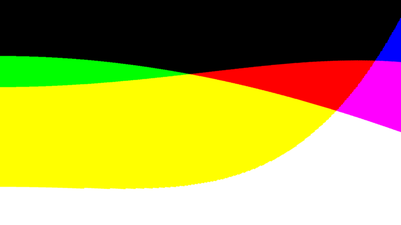
This shader shows the curves generated by random subpixel line segments on a random RGB texture (white noise).
(Note that the uneven edges of the curve are due to the fact that the interpolation takes place in the fixed-point format X.8, so the accuracy is quite limited. See the above scientific work for more information and ways to solve this problem).
Let's go ahead, indicate some values for
and and see what happens for different types of lines. m = 0, b = 0
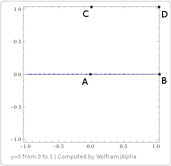
What happens if m and b are 0. In other words, what happens when sampling along the line
. Substitution of these values gives:

Interestingly, this is just linear interpolation between A and B, which makes sense when looking at a graph with a sample on a bilinear surface.
This is consistent with what Wikipedia told us: when one of the coordinates is unchanged (horizontal or vertical line), the result is linear.
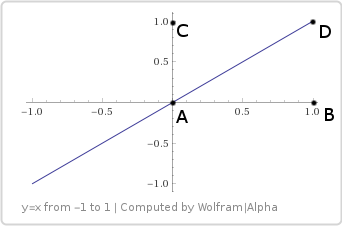
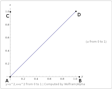
m = 1, b = 0
Let's try m = 1 and b = 0. This is the line
. The graph shows where the sample comes from on a bilinear surface: Substitution of these values gives the following equation:

We got a quadratic equation, which should not be too surprising. It is also a formula for a quadratic Bezier curve with control points
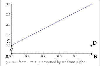
, , . m = 2, b = 1
Let's try the line
Here is the graph where we sample on a bilinear surface: Substitution of values gives us the equation:

Again, a quadratic function is obtained.
You may be surprised that the equation ends
instead but if you look at the chart, it makes sense. The line literally starts at point C when x is zero. x = 2u, y = 3u
In the above examples, we change only the variable y as a function of x. What if we also change the variable x?
One option is to enter a third variable
, which takes values from 0 to 1. Then we can express x and y through this variable. Let's see what happens if you use these two equations:


The sample runs along such a line on a bilinear surface.
Substitution of the functions u for x and y gives:

This is still a quadratic equation!
What about a quadratic trajectory?
So, now we know that when moving in a straight line on a bilinear surface, a quadratic function is obtained, except when the line is horizontal or vertical. Note: if a bilinear surface is a plane, then all the lines on this surface will be linear functions, so this is another way to get a linear result. It can also degenerate to a point. You will never get a cubic result (or higher) when moving in a straight line.
What happens if, instead of selecting along straight lines, other shapes, such as quadratic curves, are selected?
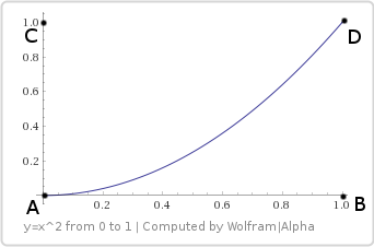
y = x * x
Let's start with the function
. Here is the curve obtained: Returning to the form of bilinear interpolation in the form of a power series, let's substitute
instead and see what happens. The initial equation is:
becomes like this:

It turns:

This is a cubic equation!
Here is a shader that draws this trajectory for random pixels: The
certain elegance of this example is that the cubic equation has four coefficients, which are based on four reference points, so that “everything goes into business,” so to speak.
This is not like sampling along linear segments where three anchor points are stored in four pixel values. One of them in this case is a little redundant.
You can use this fact, but sampling along a quadratic path to obtain a cubic curve seems like a natural approximation.
x = u * u, y = u * u
Let's see what happens if we move along x and y quadratically.
As in the linear case, we have our third variable u, which varies from 0 to 1, and we have x and y based on this variable. We will use the following equations:


The sampling path is as follows:
When we substitute the values, we obtain an equation of the fourth degree:

You may be surprised to see a linear path. It's just that x is always equal to y, even if they change non-linearly in the graph: a shader .
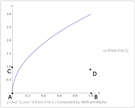
Higher order curves: x = 3u ^ 2, y = 2u ^ 4
Let's frolic a little by taking these equations:


What corresponds to such a sampling path:
If you substitute the values, then the bilinear interpolation equation ...
... turns into an equation of the sixth degree:

The Shadertoy shader generator renders it at random pixels as usual, but if u changes from 0 to 1, then x changes from 0 to 3 (y is still in the range from 0 to 1), which leads to some obvious gaps at the borders of the pixels. In a purely mathematical formulation, there wouldn’t be anything like this, but we sample on a real texture, so when we leave our safe house (0,1), we find ourselves in a completely new territory with other reference points .
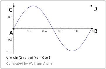
Trigonometric function: y = sin (2 * pi * x)
Let's try a function
that follows a trajectory on a bilinear surface: The bilinear interpolation equation becomes a trigonometric polynomial:

There are gaps due to going beyond the original pixel area, so in this case, this shader generated for
. It scales and shifts the y values so that they are between 0 and 1.Circle
Finally, circular sampling.


Here is its trajectory:
We substitute into the bilinear equation:

Matching Shaders .
A remarkable feature of the sample in a circle is its continuity. Notice how the left side of the curve quietly goes to the right. This seems like a pretty useful feature.
Moving on
We went a bit into the wilds, but I hope you saw many opportunities for encoding and decoding data in a very small number of pixels, if you carefully select the selection path.
This is more complicated than the simple diagonal sampling method, and shader instructions are required. In particular, in the shader, you need to encode any change in x or y before transferring linear textures to the interpolator. This means that the method requires more ALU resources. But he saves texture memory.
The last question from those listed at the beginning of the article: how will sample patterns change in higher dimensions, such as trilinear or quadrilinear interpolation?
Well, here the mechanism is about the same as in bilinear interpolation, only more measurements.
In two-dimensional bilinear interpolation, we saw that after the transformation of x and y into functions (either from each other or from the third variable u), the resulting polynomial had a degree equal to the sum of the powers of x and y.
In three dimensions with trilinear interpolation, the resulting polynomial will have a degree equal to the sum of the degrees x, y, and z.
In four dimensions with quadrilinear interpolation, add another degree z.
Consider the case when we need not a curve, but a surface or (hyper) volume.
As we saw in an extension that works with surfaces and volumes, if we have a polynomial of degree N, then it can be divided into a multidimensional polynomial (also known as a surface or hypervolume), if the sum of the degrees of each axis is added to N.
This is something about we just talked, just the opposite.
There is something that I find interesting to study in the future - to see what limitations arise if one goes too far.
For example, a 2 × 2 texture can give a quadratic function if you sample along any line in the uv coordinates. If you first express the coordinate u in terms of a cubic function, and the coordinate v in terms of another cubic function, then I think that we can make a bicubic surface.
The surface will be limited to a subset of the possible shapes of the common bicubic surface, but you will actually get a bicubic surface (there will be mostly implicit anchor points that you do not control unless you add more pixels and make additional sampling or linear interpolation of a higher dimension).
I would like to see what restrictions there are and whether there is a chance to get real benefits from something like that.
Anyway, thanks for reading! Any ideas, corrections, use cases - throw me!
@ Atrix256