Using the Python Control Systems Library to Design Automated Control Systems

Hello!

With the advent of the Python Control Systems Library [1], the solution to the basic problems of designing automatic control systems (ACS) using Python has been greatly simplified and is now almost identical to solving such problems in the mathematical package Matlab.

However, the design of control systems using this library have a number of significant features that are not in the documentation [1], therefore this publication is devoted to the features of using Python Control Systems Librar.

Let's start with the installation of the library. The documentation says about loading two slycot and control modules , in fact, for normal operation, you also need the numpy + mkl library, the rest are installed automatically when loading control .

These modules can be downloaded from the site [2]. The documentation also says that for the default interface, you just need to import the control package as follows: import control .

However, with such an import, the library does not work with any of the examples. To import the library, you must apply from control import * as for importing the matlab: from control environment . matlab import * [1].

The specialized Python Control Systems Library can only be considered in relation to the tasks of designing automatic control systems, which is why we will do so.

1. Models of system connections (tf and feedback

functions ) Input of transfer functions:

# -*- coding: utf8 -*-
from control.matlab import *
f = tf(1, [1, 1]);
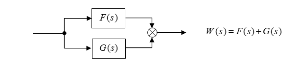
g = tf(1, [2 ,1]);

Parallel connection of blocks or systems:

# -*- coding: utf8 -*-
from control.matlab import *
f = tf(1, [1, 1]);
g = tf(1, [2 ,1]);
w = f + g
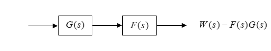
print (w)

(3 s + 2)/(s^2 + 3 s + 1)

Serial connection of blocks or systems:

# -*- coding: utf8 -*-
from control.matlab import *
f = tf(1, [1, 1]);
g = tf(1, [2 ,1]);
w = f* g
print (w)

1/(2 s^2 + 3 s + 1)

Feedback loop:



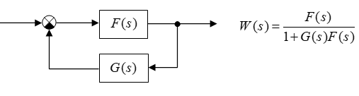
a) Negative feedback loop:

# -*- coding: utf8 -*-
from control.matlab import *
f = tf(1, [1, 1]);
g = tf(1, [2 ,1]);
w = feedback(f, g)
print(w)

(2 s + 1)/(2 s^2 + 3 s + 2)

b) Positive feedback loop:

# -*- coding: utf8 -*-
from control.matlab import *
f = tf(1, [1, 1]);
g = tf(1, [2 ,1]);
w = f/(1-f*g)
print(w)

(2 s^2 + 3 s + 1)/(2 s^3 + 5 s^2 + 3 s)

Conclusion:

Using the tf and feedback functions, you can simulate the connections of blocks and systems.

2. Dynamic and frequency characteristics of automatic control systems (ACS)

We set the transfer function of the ACS:



Find its dynamic and frequency characteristics:

# -*- coding: utf8 -*-
from control.matlab import *
""" Создадим LTI-объект с именем w, для этого выполним:"""
num= [1., 2.]
den= [3., 4., 5.,3]
w= tf(num, den)
""" Найдем полюса и нули передаточной функции с использованием команд pole, zero"""
print('Передаточная функция САУ : \n %s'%w)
print("Полюса: \n %s"%pole(w))
print("Нули:\n %s -\n "%zero(w))

Transfer function of self-propelled guns:

( s + 2)/(3 s^3 + 4 s^2 + 5 s + 3)

Poles: Build a transition function with the step (w) command:

-0.26392546+1.08251346j
-0.26392546-1.08251346j
-0. 80548241+0.j
Нули: -2

# -*- coding: utf8 -*-
from control.matlab import *
import matplotlib.pyplot as plt
""" Создадим LTI-объект с именем w, для этого выполним:"""
num= [1., 2.]
den= [3., 4., 5.,3]
w= tf(num, den)
y,x=step(w)
plt.plot(x,y,"b")
plt.title('Step Responsse ') 
plt.ylabel('Amplitude')
plt.xlabel('Time(sec)')
plt.grid(True)
plt.show()

We construct an impulse transition function using the impulse (w) command:

# -*- coding: utf8 -*-
from control.matlab import *
import matplotlib.pyplot as plt
""" Создадим LTI-объект с именем w, для этого выполним:"""
num= [1., 2.]
den= [3., 4., 5.,3]
w= tf(num, den)
y,x=impulse(w)
plt.plot(x,y,"r")
plt.title('impulse Responsse ') 
plt.ylabel('Amplitude')
plt.xlabel('Time(sec)')
plt.grid(True)
plt.show()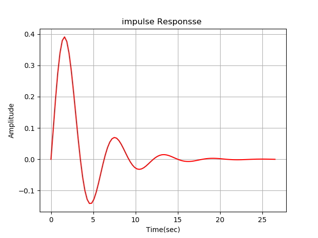

We get the Bode diagram using the bode (w) command:

# -*- coding: utf8 -*-
from control.matlab import *
import matplotlib.pyplot as plt
""" Создадим LTI-объект с именем w, для этого выполним:"""
num= [1., 2.]
den= [3., 4., 5.,3]
w= tf(num, den)
mag, phase, omega = bode(w, dB=True)
plt.plot()
plt.show()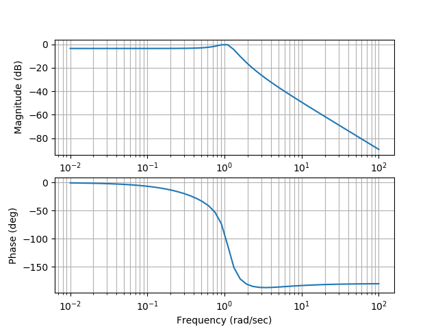

Conclusion:

Building a bode chart has some of the features shown in the listing.

Build the Nyquist diagram with the nyquist (w) command:

import matplotlib.pyplot as plt
from control.matlab import *
num= [1., 2.]
den= [3., 4., 5.,3]
w= tf(num, den)
plt.title('Nyquist Diagram ') 
plt.ylabel('Imaginary Axis')
plt.xlabel('Real Axis')
nyquist(w)
plt.grid(True)
plt.plot()
plt.show()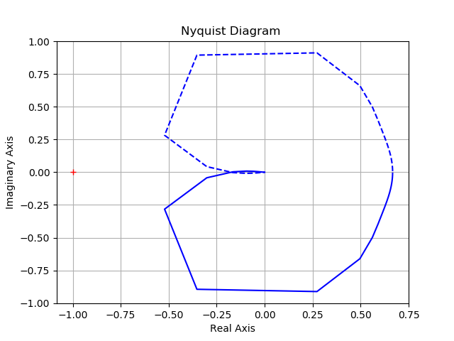

Conclusion:

Building a Nyquist diagram has some of the features shown in the listing.

We looked at simple tasks, now let's try to tune the Python Control Systems Library quite a bit.

3. Find the discrete transfer function of the actuator, the equations of state of which are of the form:

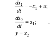(1)

To calculate, we use the matrix exponent:

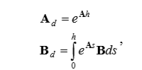(2)

where h is the quantization interval.

Find its Laplace transform from (2), which will be equal.

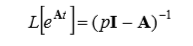(3)

where I is the identity matrix.

After substituting matrix A in (3), we obtain.

(4)

We calculate the inverse matrix.

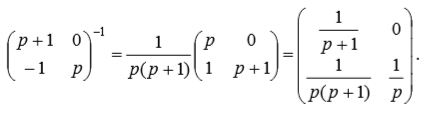(5)

Whence, carrying out the z - transformation of the last matrix, we find the transition matrix of the discrete system Ad.

(6)

where h is the time discretization interval.

The matrix Bd in accordance with (2) will be equal to.



Then a discrete analogue of the actuator model will look:

(7)

This example on the Python Control Systems Library for h = 0.1 will be written like this:

# -*- coding: utf8 -*-
import matplotlib.pyplot as plt
from control.matlab import *
import numpy as np
A=np.matrix([[-1,0],[1,0]])
B=np.matrix([[1],[0]])
C=np.matrix([[0,1]])
D=0
sn=ss(A,B,C,D)
wd=tf(sn)
print("Непрерывная модель: \n %s"%sn)
print("Передаточная функция  \n %s"%wd)
y,x=step(wd)
plt.plot(x,y,"b")
plt.title('Step Responsse ') 
plt.ylabel('Amplitude')
plt.xlabel('Time(sec)')
plt.grid(True)
plt.show()
h=1
sd=c2d(sn,h)
print("Дискретная модель : \n %s"%sd)

Transfer function

1 / (s ^ 2 + s)



Continuous model:

 A = [[-1  0]
 [ 1  0]]
B = [[1]
 [0]]
C = [[0 1]]
D = [[0]]

Discrete Model:

A = [[0.36787944 0. ]
 [0.63212056 1. ]]
B = [[0.63212056]
 [0.36787944]]
C = [[0 1]]
D = [[0]]
dt = 1

Conclusion:

Using the Python Control Systems Library, a mathematical model of the actuator based on a system of differential equations (1) was obtained. The model uses matrix operators.

I am sure that Python lovers will like the new library that significantly expands the capabilities of their favorite programming language. However, readers know that any new library requires a lot of work to adapt it to real tasks, and only after that it becomes popular and popular.

Thank you all for your attention!

References:

1. Python Control Systems.

2. Unofficial Windows Binaries for Python Extension Packages.