Volumetric atmospheric light scattering

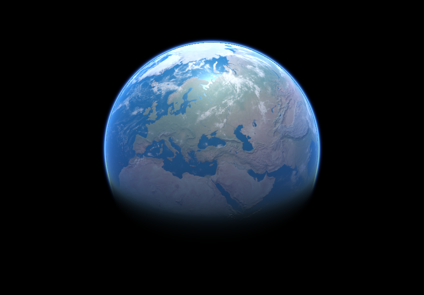
If you have lived on planet Earth long enough, you probably wondered why the sky is usually blue, but blushes at sunset. The optical phenomenon that has become the (main) reason for this is called Rayleigh scattering . In this article, I will describe how to simulate atmospheric scattering in order to simulate many of the visual effects that appear on planets. If you want to learn how to render physically accurate images of alien planets, then this tutorial is definitely worth exploring.


The article is divided into the following parts:

• Part 1. Volumetric atmospheric scattering
• Part 2. Theory of atmospheric scattering
• Part 3. Mathematics of Rayleigh scattering
• Part 4. Traveling through the atmosphere
• Part 5. Atmospheric Shader
• Part 6. Intersection of the atmosphere
• Part 7. Atmospheric dispersion shader

Part 1. Volumetric atmospheric scattering

Introduction

It is so difficult to recreate atmospheric phenomena because the sky is not an opaque object. Traditional rendering techniques assume that objects are just empty shells. All graphic calculations are performed on the surfaces of materials and do not depend on what is inside. This powerful simplification allows the rendering of opaque objects very efficiently. However, the properties of some materials are determined by the fact that light can pass through them. The final appearance of translucent objects is the result of the interaction of light with their internal structure. In most cases, this interaction can be very effectively simulated, as can be seen in the tutorial " Fast Shader for Subsurface Scattering in Unity". Unfortunately, in our case, if we want to create a convincing sky, this is not so. Instead of rendering only the" outer shell "of the planet, we have to simulate what happens to the rays of light passing through the atmosphere. Performing calculations inside an object is called volume rendering ; this subject we discussed in detail in a series of articles Volumetric Rendering in this article series, I talked about the two techniques (. raymarching and iconic function of the distance ), which can not be effectively used for the simulation of atmospheric dispersion in this article. we will look at more suitable for rendering translucent objects solid technique, often referred to as a single volumetric scattering .

Single scattering

In a room without light, we will not see anything. Objects become visible only when light rays are reflected from them and enter our eye. Most game engines (such as Unity and Unreal) assume that light moves in a "vacuum." This means that only objects can influence light. In fact, light always moves in the environment. In our case, such a medium is the air we inhale. Therefore, the distance traveled by light in air affects the appearance of an object. On the surface of the Earth, the density of air is relatively small, its influence is so insignificant that it should be taken into account only when light travels long distances. Distant mountains merge with the sky, but atmospheric dispersion has almost no effect on nearby objects.

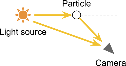
The first step in recreating the optical effect of atmospheric scattering is to analyze how light passes through media such as air. As stated above, we can only see an object when light falls into our eyes. In the context of 3D graphics, our eye is the camera used to render the scene. The molecules that make up the air around us can reflect light rays passing through them. Therefore, they are able to change the way we perceive objects. If greatly simplified, there are two ways that molecules can affect our eyesight.

Outward scattering

The most obvious way molecules interact with light is that they reflect light, changing its direction. If a ray of light directed into the camera is reflected, then we observe a process of scattering outward .


A real light source can emit quadrillion photons every second, and each of them with a certain probability can collide with an air molecule. The denser the medium in which the light moves, the more likely is the reflection of a single photon. The effect of outward scattering also depends on the distance traveled by the light.


Outward scattering leads to the fact that the light gradually becomes more and more dim, and this property depends on the distance traveled and the density of air.

Scattering inward

When light is reflected by a particle, it may happen that it is redirected to the camera. Such an effect is the opposite of outward scattering, and it is logical that it is called inward scattering .


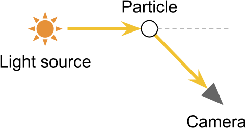
Under certain conditions, scattering inward allows you to see light sources that are not in the direct field of view of the camera. The most obvious result of this is the optical effect - light halo around light sources. They arise due to the fact that the camera receives from one source both direct and indirect rays of light, which de facto increases the number of photons received.

Unit Volumetric Scattering

One ray of light can be reflected an arbitrary number of times. This means that before you get into the camera. the beam can travel very difficult routes. This becomes a serious difficulty for us, because rendering high-quality translucent materials requires simulating the paths of each of the individual rays of light. This technique is called raytracing , and is currently too costly to implement in real time. The unit scattering technique presented in this tutorial takes into account a single light ray scattering event. Later we will see that such a simplification still allows you to get realistic results in just a small fraction of the calculations necessary for real ray tracing.

The basis of rendering a realistic sky is to simulate what happens to the rays of light when passing through the atmosphere of a planet. The diagram below shows a camera looking through a planet. The main idea of ​​this rendering technique is to calculate how light travels from$$ in $$scattering affects. This means that it is necessary to calculate the effect that the scattering in and out has on the beam passing to the camera. As stated above, due to scattering to the outside, we observe attenuation. The amount of light present at each point$$ It has a small probability of reflection away from the camera.


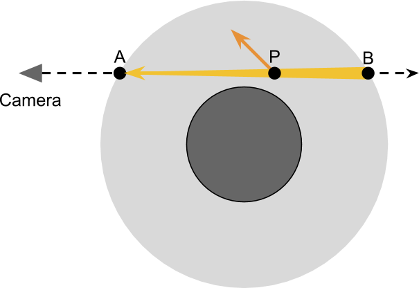
To correctly take into account the amount of outward scattering occurring at each point $$, we first need to find out how much light was present in $$. If we assume that only one star illuminates the planet, then all the light received$$must come from the sun. Part of this light will be subject to scattering inward and will be reflected in the camera:


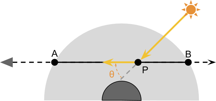
These two steps are enough to approximate most of the effects observed in the atmosphere. However, everything is complicated by the fact that the amount of light received$$ from the sun, also subject to scattering outward, when light passes through the atmosphere from $$ in $$.


To summarize what we need to do:

• The scope of the camera enters the atmosphere in $$ and is located in $$;
• As an approximation, we will take into account the effect of scattering in and out when it occurs at each point $$;
• The amount of light received $$ from the sun;
• The amount of light received $$ and subject to scattering outward when passing through the atmosphere $$;
• Part of the Light Received $$ and prone to scattering inward, which redirects the rays into the chamber;
• Part of the world from $$directed into the chamber is scattered outward and reflected from the field of view.

Part 2. Theory of atmospheric scattering

In this part, we will begin to derive the equations governing this complex but wonderful optical phenomenon.

Transmission function

To calculate the amount of light transmitted to the camera, it is useful to take the same journey that the rays from the sun pass. Looking at the diagram below, it is easy to see that the rays of light reaching$$go through empty space. Since there is nothing in their path, all the light reaches$$without undergoing any scattering effect. Let's denote the variable$$ the amount of non-scattered light received by the dot $$from the sun. During his journey to$$, the ray enters the atmosphere of the planet. Some rays collide with molecules hanging in the air and are reflected in different directions. As a result, part of the light is scattered out of the way. Amount of light reaching$$ (designated as $$) will be less than $$.


Ratio $$ and $$called pass :

$$

We can use it to indicate the percentage of light that was not scattered (i.e. was missed ) when traveling from$$ before $$. Later we explore the nature of this function. So far, the only thing we need to know is that it corresponds to the effect of atmospheric scattering outside.

Consequently, the amount of light received$$is equal to:

$$

Scatter function

Point $$receives light directly from the sun. However, not all this light passing through$$transmitted back to the camera. To calculate the amount of light actually reaching the camera, we introduce a new concept: the scattering function$$. It will denote the amount of light reflected in a certain direction. If we look at the diagram below, we will see that only rays reflected at an angle will be directed to the camera$$.


Value $$ denotes the fraction of light reflected on $$radian. This function is our main problem, and we will examine its nature in the next part. So far, the only thing you need to know is that it depends on the color of the light received (determined by the wavelength$$), scattering angle$$and heights$$ points $$. Altitude is important because atmospheric density varies as a function of altitude. And density is one of the factors determining the amount of light scattered.

Now we have all the necessary tools for writing a general equation showing the amount of light transmitted from$$ to $$:

$$

Thanks to the previous definition, we can expand $$:

$$

$$

The equation speaks for itself:

• Light travels from the sun to $$without scattering in the vacuum of space;
• Light enters the atmosphere and passes from $$ to $$. In this process, due to the scattering outward only part$$ reaches the destination;
• Part of the light that got from the sun to $$reflected back to the camera. The fraction of light subject to inward scattering is$$;
• The remaining light passes from $$ before $$, and again only part $$.

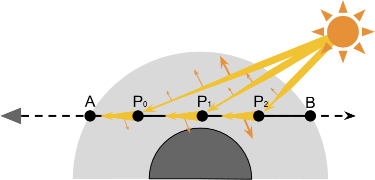
Numerical integration

If you carefully read the previous paragraphs, you might notice that the brightness was recorded in different ways. Symbol$$ denotes the amount of light transmitted from $$ to $$. However, the value does not take into account all the light that receives$$. In these simplified models of atmospheric scattering, we take into account scattering inward from each point along the field of view of the camera in the atmosphere.

The total amount of light received$$ ($$), is calculated by adding up the influence of all points $$. From the point of view of mathematics, on the segment$$there are an infinite number of points; therefore, cyclic traversal of all of them is impossible. However we can divide$$ for smaller lengths $$ (see diagram below), and summarize the impact of each of them.


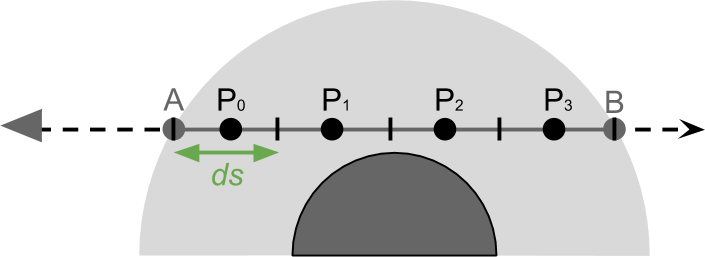
Such an approximation process is called numerical integration and leads to the following expression:

$$

The more points we take into account, the more accurate the final result will be. In reality, in our atmospheric shader, we simply cycle around several points$$ inside the atmosphere, summing up their influence in the overall result.

Directional lighting

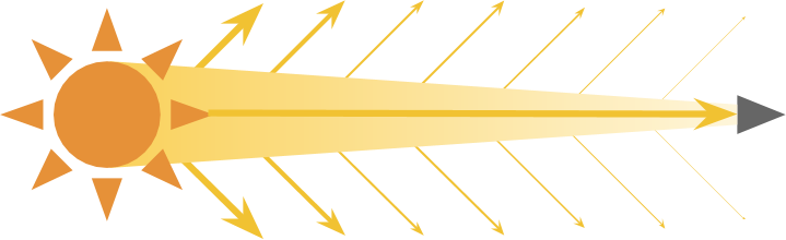
If the sun is relatively close, then it is best to model it as a point source of light . In this case, the amount received$$light depends on the distance to the sun. However, if we are talking about planets, we often assume that the sun is so far away that its rays fall on the planet at one angle. If this is true, then we can model the sun as a directional light source . The light received from a directional light source remains constant, regardless of the distance traveled by it. Therefore every point$$ receives the same amount of light, and the direction relative to the sun is the same for all points.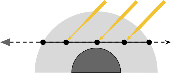


We can use this assumption to simplify our equations.

Let's replace$$ constant $$, which determines the brightness of the sun .

$$

$$

$$

There is another optimization we can perform, it includes a scatter function $$. If sunlight always falls from one direction, then the angle$$becomes permanent. Below we will see that directed influence can be excluded from the amount$$. But for now, we will leave him.

Absorption coefficient

In describing the possible results of the interaction between light and air molecules, we allowed only two options - either through and through, or reflection. But there is a third possibility. Some chemical compounds absorb light. There are many substances in the Earth’s atmosphere that have this property. Ozone, for example, is in the upper atmosphere and actively interacts with ultraviolet radiation. However, its presence has practically no effect on the color of the sky, because it absorbs light outside the visible spectrum. Here on Earth, the effects of light-absorbing substances are often ignored. But in the case of other planets it is impossible to refuse it. For example, the usual coloration of Neptune and Uranus is caused by the presence of a large amount of methane in their atmosphere. Methane absorbs red light, which gives a blue tint.

Часть 3. Математика рэлеевского рассеяния.

In this part, we will get acquainted with the mathematics of Rayleigh scattering - an optical phenomenon due to which the sky looks blue. The equations derived in this part of the equation will be transferred to the shader code of the next part.

Introduction

In the previous part, we derived an equation that provides a good basis for approximating atmospheric scattering in a shader. However, we have missed the fact that one equation will not give us convincing results. If we need a beautiful looking atmospheric shader, then we need to go a little deeper into mathematics.

The interaction between light and matter is incredibly complex, and we will not be able to fully describe it in an easy way. Actually, modeling atmospheric scattering is very time consuming. Part of the problem is that the atmosphere is not a homogeneous environment. Its density and composition vary significantly as a function of height, which makes it almost impossible to create an “ideal” model.

That is why several scattering models are given in the scientific literature, each of which is intended to describe a subset of the optical phenomena that arise under certain conditions. Most of the optical effects demonstrated by the planets can be recreated, taking into account only two different models: Rayleigh scattering and scattering of light by a spherical particle . These two mathematical tools make it possible to predict light scattering on objects of various sizes. The first models the reflection of light by oxygen and nitrogen molecules, which make up most of the air. The latter models the reflection of light in larger structures present in the lower atmosphere, such as pollen, dust and pollutants.

Rayleigh scattering is the cause of blue sky and red sunsets. Scattering of light by a spherical particle gives the clouds their white color. If you want to know how this happens, then we will have to dive deeper into the mathematics of scattering.

Rayleigh scattering

What is the fate of a photon striking a particle? To answer this question, we need to rephrase it more formally. Imagine that a ray of light passes through an empty space and suddenly collides with a particle. The result of such a collision is highly dependent on the particle size and color of the light beam. If the particle is small enough (the size of atoms or molecules), then the behavior of light is better predicted using Rayleigh scattering .

What is going on? Part of the world continues its journey, “not feeling” any influence. However, a small percentage of this source light interacts with the particle and scatters in all directions. However, not all directions receive the same amount of light. Photons are more likely to pass directly through the particle or bounce back. That is, the photon reflection option is 90 degrees less large. This behavior can be seen in the diagram below. The blue line shows the most likely directions of the scattered light.


This optical phenomenon is mathematically described by the Rayleigh scattering equation$$that gives us a share of the source light $$reflected in the direction $$:

$$

$$

Where:

• $$: wavelength of the incoming light;
• $$: Angle rasseiyaniya (scattering angle) ;
• $$: высота (altitude) точки;
• $$: коэффициент преломления воздуха;
• $$: количество молекул на кубический метр стандартной атмосферы;
• $$: коэффициент плотности.Это число на уровне моря равно $$, и экспоненциально уменьшается с увеличением $$. Об этой функции можно многое сказать, и мы рассмотрим её в следующих частях.

The first thing that can be seen in Rayleigh scattering is that in some directions more light travels than in others. The second important aspect is that the amount of scattered light is highly dependent on the wavelength.$$coming light. The pie chart below renders$$for three different wavelengths. Calculation$$ at $$often called sea ​​level scattering .


The figure below shows the visualization of the scattering coefficients for the continuous wavelength / color range of the visible spectrum (the code is available in ShaderToy ).


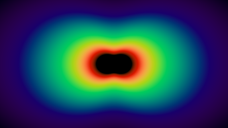
The center of the image appears black because the wavelengths in this range are outside the visible spectrum.

Rayleigh scattering coefficient

The Rayleigh scattering equation shows how much light is scattered in a certain direction. However, it does not tell us how much energy has been dissipated. To calculate this, we need to take into account energy dissipation in all directions. The derivation of the equation is not easy; if you haven’t mastered complex matanalysis, here is the result:

$$

Where $$shows the fraction of energy that is lost due to scattering after a collision with a single particle. Often this value is called the Rayleigh scattering coefficient .

If you read the previous part of the tutorial, you can guess that$$is actually the attenuation coefficient that was used in determining the transmittance$$ on the segment $$.

Unfortunately, the calculation$$very expensive. In the shader that we are going to write, I will try to save as many calculations as possible. For this reason, it will be useful to “extract” from the scattering coefficient all factors that are constants. What gives us$$, which is called the Rayleigh scattering coefficient at sea level ($$):

$$

This new equation gives us another way to understand how different colors are scattered. The graph below shows the amount of scattering to which light is exposed, as a function of its wavelength.


This is a strong relationship between the scattering coefficient. $$ and $$which causes a red sky at sunset. Photons received from the sun are distributed over a wider range of wavelengths. Rayleigh scattering tells us that the atoms and molecules of the Earth’s atmosphere scatter blue more than green or red. If the light can move long enough, then its entire blue component will be lost due to scattering. This is what happens at sunset, when the light travels almost parallel to the surface.

Reasoning the same way, we can understand why the sky looks blue. The light of the sun is falling from one direction. However, its blue component is scattered in all directions. When we look at the sky, blue light comes from all directions.

Rayleigh phase function

The original equation describing Rayleigh scattering, $$, can be decomposed into two components. The first is the scattering coefficient we just derived$$which modulates its intensity. The second part is related to the scattering geometry, and controls its direction:

$$

This new value $$ can be obtained by dividing $$ on the $$:

$$

$$

$$

You can see that this new expression is independent of the wavelength of the incoming light. This seems counterintuitive because we know for sure that Rayleigh scattering affects shortwaves more strongly.

However$$models the shape of the dipole that we saw above. Member$$ serves as a normalization coefficient so that the integral over all possible angles $$ summed up in $$. If formulated technically, we can say that the integral over$$ steradians equal $$.

In the following parts, we will see how the separation of these two components allows us to derive more efficient equations.

To summarize

• Rayleigh scattering equation : indicates the fraction of light reflected in the direction$$. The amount of scattering depends on the wavelength.$$ incoming light.

$$

Moreover:

$$

• Rayleigh scattering coefficient : indicates the fraction of light lost due to scattering after the first collision.

$$

• Rayleigh scattering coefficient at sea level : this is an analog$$. Creating this additional coefficient will be very useful for deriving more efficient equations.

$$

If we consider wavelengths roughly corresponding to the red, green, and blue colors, we will obtain the following results:

$$

$$

$$

These results are calculated under the assumption that $$ (this implies that $$) This only happens at sea level, where the dispersion coefficient has a maximum value. Therefore, it serves as a "guide" for the amount of light scattering.

• Rayleigh phase function : controls the scattering geometry, which denotes the relative fraction of light lost in a particular direction. Coefficient$$ serves as a normalization coefficient, therefore, the integral over the unit sphere will be $$.

$$

• Density coefficient : This function is used to simulate the density of the atmosphere. Its formal definition will be presented below. If you are not against mathematical spoilers, then it is defined as follows:

$$

Where $$meters is called the reduced height .

Part 4. Travel through the atmosphere.

In this part, we will consider modeling atmospheric density at different heights. This is a necessary step, because the density of the atmosphere is one of the parameters necessary for the correct calculation of Rayleigh scattering.

Atmospheric density coefficient

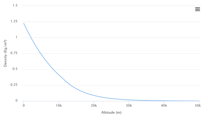
So far, we have not considered the role of the atmospheric density coefficient $$. It is logical that the scattering force is proportional to the density of the atmosphere. The more molecules per cubic meter, the greater the probability of scattering of photons. The difficulty is that the structure of the atmosphere is very complex, it consists of several layers with different pressure, density and temperature. Fortunately for us, the bulk of Rayleigh scattering occurs in the first 60 km of the atmosphere. In the troposphere, temperature decreases linearly, and pressure decreases exponentially.

The diagram below shows the relationship between density and height in the lower atmosphere.


Value $$ is a measurement of the atmosphere at altitude $$meters, normalized in a way that starts from zero. In many scientific articles$$also called the density coefficient , because it can also be defined as follows:

$$

Dividing the true density by $$we get that $$ at sea level is equal $$. However, as emphasized above, the calculation$$far from nontrivial. We can approximate it as an exponential curve; some of you could already understand that the density in the lower atmosphere is decreasing exponentially .

If we want to approximate the density coefficient through an exponential curve, then we can do this as follows:

$$

Where $$Is a scale factor called the reduced height . For Rayleigh scattering in the lower atmosphere of the Earth, it is often believed that$$meters (see diagram below). For scattering light by a spherical particle, the value is often approximately equal$$ meters.


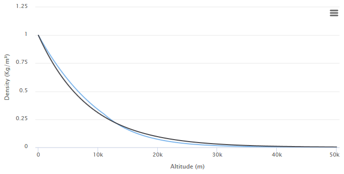
The value used for $$does not give the best approximation $$. However, this is actually not a problem. Most of the values ​​presented in this tutorial undergo serious approximations. To create visually pleasing results, it will be much more efficient to adjust the available parameters to the reference images.

Exponential decrease

In the previous part of the tutorial, we derived an equation showing us how to account for the outward scattering to which a ray of light is exposed after interacting with an individual particle. The value used to model this phenomenon was called the scattering coefficient$$. To take it into account, we introduced the coefficients$$.

In the case of Rayleigh scattering, we also derived a closed form for calculating the amount of light subject to atmospheric scattering in a single interaction:

$$

When calculating at sea level, i.e. when $$, the equation gives the following results:

$$

$$

$$

Where $$, $$ and $$- wavelengths roughly corresponding to red, green and blue.

What is the meaning of these numbers? They represent the fraction of light that is lost in a single interaction with a particle. Assuming that a ray of light initially has brightness$$ and passes a segment of the atmosphere with a (general) scattering coefficient $$, then the amount of light remaining after scattering is:

$$

This is true for a single collision, but we are interested in what kind of energy is dissipated during a certain distance. This means that the remaining light undergoes this process at every point.

When light passes through a homogeneous medium with a scattering coefficient$$, how can we calculate how much of it will remain when moving a certain distance?

For those of you who have studied matanalysis, this may seem familiar. When a multiplicative process is repeated on a continuous segment$$then the Euler number enters the scene . The amount of light remaining after scattering after passage$$ meters equals:

$$

And again, we are faced with an exponential function. It has nothing to do with the exponential function describing the density coefficient$$. Both phenomena are described by exponential functions because they are both subject to exponential reduction. Other than that, there is no connection between them.

Uniform transmittance

In the second part of the tutorial we introduced the concept of transmission$$as the fraction of light remaining after the scattering process when passing through the atmosphere. Now we have all the elements to deduce the equation describing it.

Let's look at the diagram below and think about how to calculate the transmittance for the segment$$. You can easily see that the rays of light reaching$$pass through empty space. Therefore, they are not scattered. Consequently, the amount of light in$$actually equal to the brightness of the sun$$. During this journey to$$part of the light is scattered out of the way; therefore the amount of light reaching$$ ($$) will be less than $$.


The amount of scattered light depends on the distance traveled. The longer the path, the greater the attenuation. According to the law of exponential reduction, the amount of light at a point$$ can be calculated as follows:

$$

Where $$ - the length of the segment from $$ before $$, a $$- exponential function$$.

Atmospheric transmission

We based our equation on the assumption that the probability of reflection ( scattering coefficient$$ same at every point along $$. Unfortunately, this is not the case.

The scattering coefficient is highly dependent on the density of the atmosphere. The more air molecules per cubic meter, the higher the chance of a collision. The density of the planet’s atmosphere is heterogeneous, and varies with altitude. It also means that we cannot calculate outward scatterings from$$in one step. To solve this problem, we need to calculate the outward dispersion at each point using the scattering coefficient.

To understand how this works, let's start with the approximation. Section$$ divided into two $$ and $$.


First we calculate the amount of light from $$which reaches $$:

$$

Then we use the same approach to calculate the amount of light reaching $$ of $$:

$$

If we substitute $$ into the second equation and simplify, we get:


If $$ and $$ have the same length $$, then we can simplify the expression even more: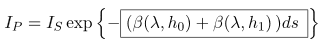


In the case of two segments of the same length with different scattering coefficients, the outward scattering is calculated by summing the scattering coefficients of the individual segments and multiplied by the lengths of the segments.

We can repeat this process with an arbitrary number of segments, getting closer and closer to the true value. This will lead us to the following equation:

$$

Where $$ - point height $$.

The method of dividing a straight line into many segments, which we just used, is called numerical integration .

If we assume that the initial amount of light received is$$, then we obtain the equation of atmospheric transmission through an arbitrary segment:

$$

We can expand this expression even further. replacing the total$$ the real value used in Rayleigh scattering, $$:

$$

Many factors $$ constant, so that they can be carried out for the amount of:

$$

The value expressed by summation is called the optical thickness$$which we will calculate in the shader. The remainder is a magnification factor that can only be calculated once, and it corresponds to a scattering coefficient at sea level . In the finished shader, we will only calculate the optical thickness, and the scattering coefficients at sea level$$We will transmit as input.

Summarize:

$$

Part 5. Atmospheric shader.

Introduction

Writing shader

We can start writing a shader for this effect in an infinite number of ways. Since we want to render atmospheric scattering on planets, it is logical to assume that it will be used on spheres.

If you use this tutorial to create a game, chances are that you will apply a shader to an existing planet. Adding atmospheric scatter calculations on top of the swatch is possible, but usually produces poor results. The reason is that the atmosphere is larger than the radius of the planet, so it needs to be rendered on a transparent sphere of a slightly larger size. The figure below shows how the atmosphere extends over the surface of the planet, mixing with the empty space behind it.


The application of dispersible material to a separate sphere is possible, but redundant. In this tutorial, I suggest expanding Standard Surface Shader Unity by adding a shader pass that renders the atmosphere in a slightly larger sphere. We will call it the atmospheric sphere .

Two-pass shader

If you used to work with Unity surface shaders , you may have noticed that they do not support a block Pass, with which several passes are set in the vertex and fragment shaders .

Creating a shader with two passes is possible, just add two separate sections of the CG code in one block SubShader:

Shader "Custom/NewSurfaceShader" {
 Properties {
 _Color ("Color", Color) = (1,1,1,1)
 _MainTex ("Albedo (RGB)", 2D) = "white" {}
 _Glossiness ("Smoothness", Range(0,1)) = 0.5
 _Metallic ("Metallic", Range(0,1)) = 0.0
 }
 SubShader {
 // --- Первый проход ---
 Tags { "RenderType"="Opaque" }
 LOD 200
 CGPROGRAM
 // Здесь код Cg
 ENDCG
 // ------------------
 // --- Второй проход ---
 Tags { "RenderType"="Opaque" }
 LOD 200
 CGPROGRAM
 // Здесь код Cg
 ENDCG
 // -------------------
 }
 FallBack "Diffuse"
}

You can change the first pass to render the planet. From now on, we will focus on the second pass, realizing atmospheric scattering in it.

Normal Extrusion

The atmospheric sphere is slightly larger than the planet. This means that the second pass should extrude the sphere out. If your model uses smooth normals, then we can achieve this effect using a technique called extrusion of normals .

Normal extrusion is one of the oldest shader tricks, and is usually one of the first to be studied. My blog has many references to it; A good start might be a Surface Shader post from the A Gentle Introduction to Shaders series .

If you are unfamiliar with how the extrusion of normals works, then I will explain: all the vertices are processed by the shader using its vertex function. We can use this function to change the position of each vertex, making the sphere bigger.

The first step is to change the directive by pragmaadding it vertex:vert; this will force Unity to execute a function for each vertex vert.

#pragma surface surf StandardScattering vertex:vert
void vert (inout appdata_full v, out Input o)
{
 UNITY_INITIALIZE_OUTPUT(Input,o);
 v.vertex.xyz += v.normal * (_AtmosphereRadius - _PlanetRadius);
}

This code fragment shows a vertex function extruding a sphere along its normals. The magnitude of the extrusion of a sphere depends on the size of the atmosphere and the size of the planet. Both of these values ​​need to be passed to the shader as properties that can be accessed through the material inspector .

Our shader also needs to know where the center of the planet is. We can add its calculation to the vertex function too. We discussed the finding of the center point of an object in the space of the world in the article Vertex and Fragment Shaders .

struct Input
{
 float2 uv_MainTex;
 float3 worldPos; // Автоматически инициализируется Unity
 float3 centre;   // Инициализируется в вершинной функции
};
void vert (inout appdata_full v, out Input o)
{
 UNITY_INITIALIZE_OUTPUT(Input,o);
 v.vertex.xyz += v.normal * (_AtmosphereRadius - _PlanetRadius);
 o.centre = mul(unity_ObjectToWorld, half4(0,0,0,1));
}

Аддитивное смешивание

Another interesting feature that we need to deal with is transparency. Usually transparent material allows you to see what is behind the object. This solution in our case will not work, because the atmosphere is not just a transparent piece of plastic. Light passes through it, so we need to use the additive mixing mode to increase the luminosity of the planet.

In the standard Unity Surface Shader, no blending mode is enabled by default. To change the situation, we will have to replace the labels in the second pass with the following:

Tags { "RenderType"="Transparent"
 "Queue"="Transparent"}
LOD 200
Cull Back
Blend One One

The expression is Blend One Oneused by the shader to access the additive blending mode.

Native lighting function

Most often, when writing a surface shader, programmers change its function surf, which is used to provide “physical” properties, such as albedo, surface smoothness, metal properties, etc. All these properties are then used by the shader to calculate realistic shading.

In our case, these calculations are not required. To get rid of them, we need to remove the lighting model used by the shader . I examined this topic in detail; You can study the following posts to figure out how to do this:

• 3D Printer Shader Effect ( translation on Habré)
• CD-ROM Shader: Diffraction Grating
• Fast Subsurface Scattering in Unity ( Habré translation )

The new lighting model will be called StandardScattering; we must create a function for lighting in real time and for global illumination, that is, respectively, LightingStandardScatteringand LightingStandardScattering_GI.

The code that we need to write will also use properties such as the direction of lighting and the direction of view . They can be obtained using the following code snippet.

#pragma surface surf StandardScattering vertex:vert
#include "UnityPBSLighting.cginc"
inline fixed4 LightingStandardScattering(SurfaceOutputStandard s, fixed3 viewDir, UnityGI gi)
{
 float3 L = gi.light.dir;
 float3 V = viewDir;
 float3 N = s.Normal;
 float3 S = L; // Направление освещения от солнца
 float3 D = -V;  // Направление луча видимости, проходящего через атмосферу
 ...
}
void LightingStandardScattering_GI(SurfaceOutputStandard s, UnityGIInput data, inout UnityGI gi)
{
 LightingStandard_GI(s, data, gi); 
}

It ...will contain the shader code itself, which is needed to implement this effect.

Floating point precision

In this tutorial we will assume that all calculations are performed in meters. This means that if we need to simulate the Earth, then we need a sphere with a radius of 6371000 meters. In fact, in Unity this is not possible due to floating point errors that occur when you have to work with very large and very small numbers at the same time.

To circumvent these limitations, you can scale the scattering coefficient to compensate. For example, if the planet has a radius of only 6.371 meters, then the scattering coefficient
$$ should be more than 1,000,000 times, and the reduced height $$- 1,000,000 times less.

In my Unity project, all properties and calculations are expressed in meters. This allows us to use real, physical values ​​for the scattering coefficients and the reduced height. However, the shader also gets the size of the sphere in meters, so that it can perform scale conversion from Unity units to real-scale meters.

Part 6. Intersection of the atmosphere.

As mentioned above, the only way to calculate the optical thickness of a segment passing through the atmosphere is through numerical integration . This means that you need to divide the interval into smaller lengths$$ and calculate the optical thickness of each, considering its density constant.


Above is the optical thickness. $$It is calculated by four samples, each of which takes into account the density in the center of the segment itself.

The first step will obviously be finding the points$$ and $$. If we assume that the objects we render are a sphere, then Unity will try to render its surface. Each pixel on the screen corresponds to a point on the sphere. In the figure below, this point is called$$(from origin ). In the surface shader$$corresponds to a variable worldPosin the structure Input. This is the amount of work the shader does; the only information available to us is$$direction $$, which indicates the direction of the line of sight , and the atmospheric sphere centered$$ and radius $$. The difficulty lies in computing$$ and $$. The geometry will be used the fastest, reducing the problem to finding the intersection of the atmospheric sphere and the camera visibility beam .


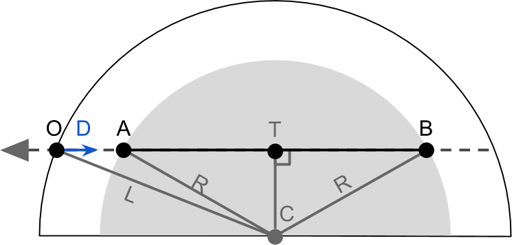
Firstly, it is worth noting that $$, $$ and $$lie on the line of sight. This means that we can handle their position not as a point in 3D space, but as with the distance of the line of sight to origin.$$Is the real point (represented as in the shader float3), and$$ - distance to the starting point $$(stored as float).$$ and $$ - two equally correct ways of designating the same point, that is, it is true:

$$

$$

where is the entry with a bar above $$ denotes the length of the segment between two arbitrary points $$ and $$.

In the shader code for efficiency we will use$$ and $$, and compute them from $$:

$$

$$

It is also worth noting that the segments $$ and $$have the same length. Now, to find the intersection points, we need to calculate$$ and $$.

Section$$The easiest way to calculate. If you look at the diagram above, you can see that$$ is a projection of a vector $$on the line of sight. Mathematically, this projection can be done using a scalar product . If you are familiar with shaders, then you may know that a scalar product is a measure of how “aligned” two directions are. When it is applied to two vectors, and one of them has a unit length, it becomes the projection operator:

$$

It is also worth noting that
$$ Is a three-dimensional vector, not the length of the segment between $$ and $$.

Next we need to calculate the length of the segment$$. It can be calculated using the Pythagon theorem in a triangle$$. She claims that:

$$

And that means that:

$$

Length $$still unknown. However, it can be calculated by again applying the Pythagorean theorem to the triangle$$:

$$

$$

Now we have all the necessary quantities. Summarize:

$$

$$

$$

$$

$$

There are square roots in this set of equations. They are defined only for non-negative numbers. If$$, then there is no solution, which means that the line of sight does not intersect with the sphere.

We can convert this to the following Cg function:

bool rayIntersect
(
 // Ray
 float3 O, // Origin
 float3 D, // Направление
 // Сфера
 float3 C, // Центр
 float R, // Радиус
 out float AO, // Время первого пересечения
 out float BO  // Время второго пересечения
)
{
 float3 L = C - O;
 float DT = dot (L, D);
 float R2 = R * R;
 float CT2 = dot(L,L) - DT*DT;
 // Точка пересечения за пределами круга
 if (CT2 > R2)
 return false;
 float AT = sqrt(R2 - CT2);
 float BT = AT;
 AO = DT - AT;
 BO = DT + BT;
 return true;
}

It returns not one, but three values $$, $$as well as the binary value of the intersection. The lengths of these two segments are returned using keywords outthat save after the function completes any changes that it made to these parameters.

Collision with the planet

There is another problem to consider. Some rays of visibility collide with the planet, so their journey through the atmosphere ends early. One solution is to revise the above.

A simpler but less effective approach is to perform rayIntersecttwice and change the endpoint if necessary.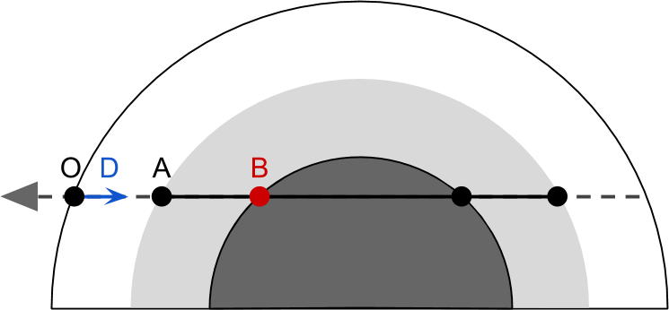


This translates to the following code:

// Пересечения с атмосферной сферой
float tA; // Точка входа в атмосферу (worldPos + V * tA)
float tB; // Точка выхода из атмосферы  (worldPos + V * tB)
if (!rayIntersect(O, D, _PlanetCentre, _AtmosphereRadius, tA, tB))
 return fixed4(0,0,0,0); // Лучи видимости смотрят в глубокий космос
// Проходит ли луч через ядро планеты?
float pA, pB;
if (rayIntersect(O, D, _PlanetCentre, _PlanetRadius, pA, pB))
 tB = pA;

Part 7. Atmospheric dispersion shader.

In this part, we will finally complete the work on simulating Rayleigh scattering in the atmosphere of the planet.

Visibility Beam Sampling

Let's recall the equation of atmospheric scattering that we recently derived:

$$

The amount of light we receive is equal to the amount of light emitted by the sun, $$multiplied by the sum of the individual influences of each point $$ on the segment $$.

We can implement this function directly in the shader. However, some optimizations need to be made here. In the previous part, I said that the expression can be simplified even more. The first thing to do is to break up the scattering function into two main components:

$$

Phase function$$and sea ​​level dispersion coefficient$$ are constant with respect to the sum, because the angle $$ and wavelength $$independent of the sampled point. Therefore, they can be carried out for the amount of:

$$

This new expression is mathematically similar to the previous one, but more efficient in calculating, because the most "heavy" parts are derived from the sum.

We are not yet ready for its implementation. There are an infinite number of points$$which we must consider. Reasonable approximation$$ will be a split $$ into several shorter segments $$and the addition of the influence of each individual segment. Having done so, we can assume that each segment is small enough to have a constant density. In general, this is not so, but if$$ small enough, then we can achieve a fairly good approximation.


The number of segments in $$we will call the samples of visibility because all segments lie on the line of sight. In the shader, this will be a property _ViewSamples. Since this property, we can access it from the material inspector. This allows us to reduce the accuracy of the shader for its performance.

The following code snippet allows you to bypass all segments in the atmosphere.

// Численное интегрирование для вычисления
// влияния света в каждой точке P отрезка AB
float3 totalViewSamples = 0;
float time = tA;
float ds = (tB-tA) / (float)(_ViewSamples);
for (int i = 0; i < _ViewSamples; i ++)
{
 // Позиция точки
 // (сэмплирование в середине отрезка сэмпла видимости)
 float3 P = O + D * (time + ds * 0.5);
 // T(CP) * T(PA) * ρ(h) * ds
 totalViewSamples += viewSampling(P, ds);
 time += ds;
}
// I = I_S * β(λ) * γ(θ) * totalViewSamples
float3 I = _SunIntensity *  _ScatteringCoefficient * phase * totalViewSamples;

The variable is timeused to track how far we are from the starting point.$$. After each iteration, it increases by ds.

Optical Thickness PA

Every point on the line of sight $$contributes to the final color of the pixel we draw. This contribution, expressed mathematically, is a value inside the sum:

$$

Let's try to simplify this expression, as in the last paragraph. We can further expand the above expression by replacing$$ its definition:

$$

Result of skipping over $$ and $$ turns into:

$$

$$

$$

The combined transmission is modeled as an exponential decrease, the coefficient of which is the sum of the optical thicknesses along the path traveled by light ($$ and $$) times the dispersion coefficient at sea level ($$ at $$)
The first value that we begin to calculate is the optical thickness of the segment$$, which goes from the point of entry into the atmosphere to the point at which we are currently sampling in the for loop. Let's recall the definition of optical thickness:

$$

If we had to implement it “forehead”, then we would create a function opticalDepththat samples the points between$$ and $$. It is possible, but very inefficient. In fact,$$Is the optical thickness of the line segment that we are already analyzing in the outermost for loop. We can save a lot of calculations if we calculate the optical thickness of the current segment centered in$$( opticalDepthSegment), and continue to summarize it in a for ( opticalDepthPA) loop .

// Накопитель оптической толщины
float opticalDepthPA = 0;
// Численное интегрирование для вычисления
// влияния света каждой точки P в AB
float time = tA;
float ds = (tB-tA) / (float)(_ViewSamples);
for (int i = 0; i < _ViewSamples; i ++)
{
 // Позиция точки
 // (сэмплируется посередине сэмпла отрезка видимости)
 float3 P = O + D * (time + viewSampleSize*0.5);
 // Оптическая толщина текущего отрезка
 // ρ(h) * ds
 float height = distance(C, P) - _PlanetRadius;
 float opticalDepthSegment = exp(-height / _ScaleHeight) * ds;
 // Накопление оптических толщин
 // D(PA)
 opticalDepthPA += opticalDepthSegment;
 ... 
 time += ds;
}

Light sampling

If we return to the expression for the influence of light $$, then the only necessary value is the optical thickness of the segment $$,

$$

We will move the code that calculates the optical thickness of the segment $$into a function called lightSampling. The name is taken from a ray of light , which is a segment starting at$$and directed towards the sun. We called the point at which it comes out of the atmosphere$$.

However, the function lightSamplingdoes not just calculate the optical thickness$$. So far we have considered only the influence of the atmosphere and ignored the role of the planet itself. Our equations do not take into account the possibility that a ray of light moving from$$to the sun, may collide with the planet. If this happens, then all calculations performed up to this point are not applicable, because the light does not actually reach the camera.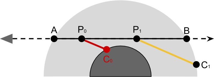


In the diagram below it is easy to see that the influence of light $$ must be ignored because no light of the sun reaches $$. When cycling through points between$$ and $$The function lightSamplingalso checks for collisions with the planet. This can be done by checking the height of the point for negativity.

bool lightSampling
( float3 P, // текущая точка внутри атмосферной сферы
 float3 S, // Направление к солнцу
 out float opticalDepthCA
)
{
 float _; // это нас не интересует
 float C;
 rayInstersect(P, S, _PlanetCentre, _AtmosphereRadius, _, C);
 // Сэмплы на отрезке PC
 float time = 0;
 float ds = distance(P, P + S * C) / (float)(_LightSamples);
 for (int i = 0; i < _LightSamples; i ++)
 {
 float3 Q = P + S * (time + lightSampleSize*0.5);
 float height = distance(_PlanetCentre, Q) - _PlanetRadius;
 // Внутри планеты
 if (height < 0)
 return false;
 // Оптическая толщина для луча света
 opticalDepthCA += exp(-height / _RayScaleHeight) * ds;
 time += ds;
 }
 return true;
}

The function above calculates the point first $$with the help of rayInstersect. Then she divides the segment$$into segments _LightSamplesof length ds. The calculation of optical thickness is the same as that used in the outermost loop.

The function returns false if a collision with a planet occurs. We can use this to update the missing code of the outermost loop by replacing ....

 // D(CP)
 float opticalDepthCP = 0;
 bool overground = lightSampling(P, S);
 if (overground)
 {
 // Комбинированное пропускание
 // T(CP) * T(PA) = T(CPA) = exp{ -β(λ) [D(CP) + D(PA)]}
 float transmittance = exp
 (
 -_ScatteringCoefficient *
 (opticalDepthCP + opticalDepthPA)
 );
 // Влияния света
 // T(CPA) * ρ(h) * ds
 totalViewSamples += transmittance * opticalDepthSegment;
 }

Now that we have taken into account all the elements, our shader is ready.

[Note per .: on the author’s Patreon page, you can buy access to Standard and Premium versions of the finished shader.]