Car Brand Ratings: An Example of Multiple Response Variable Analysis

In questionnaire marketing research quite often there are questions in which respondents can choose several suitable options from the list of possible answers (check all that apply questions). Respondents to such questions are asked by variables with multiple response (multiple-response variables). Suitable statistical methods for working with multiple-response variables are not widely known. In this article, we will analyze the analysis of such variables using the example of automobile ratings data.

Data

This is a typical example of a question in a questionnaire that allows for multiple responses from the Customer Satisfaction Survey Template. Source: Survey Monkey

We will use automobile ratings data in this article (Van Gysel 2011). They are freeware and are included in the plfm R package . These data should be taken only as an object to demonstrate mathematical methods and visualization tools. Do not assume that the results are based on a full representative survey of a group.

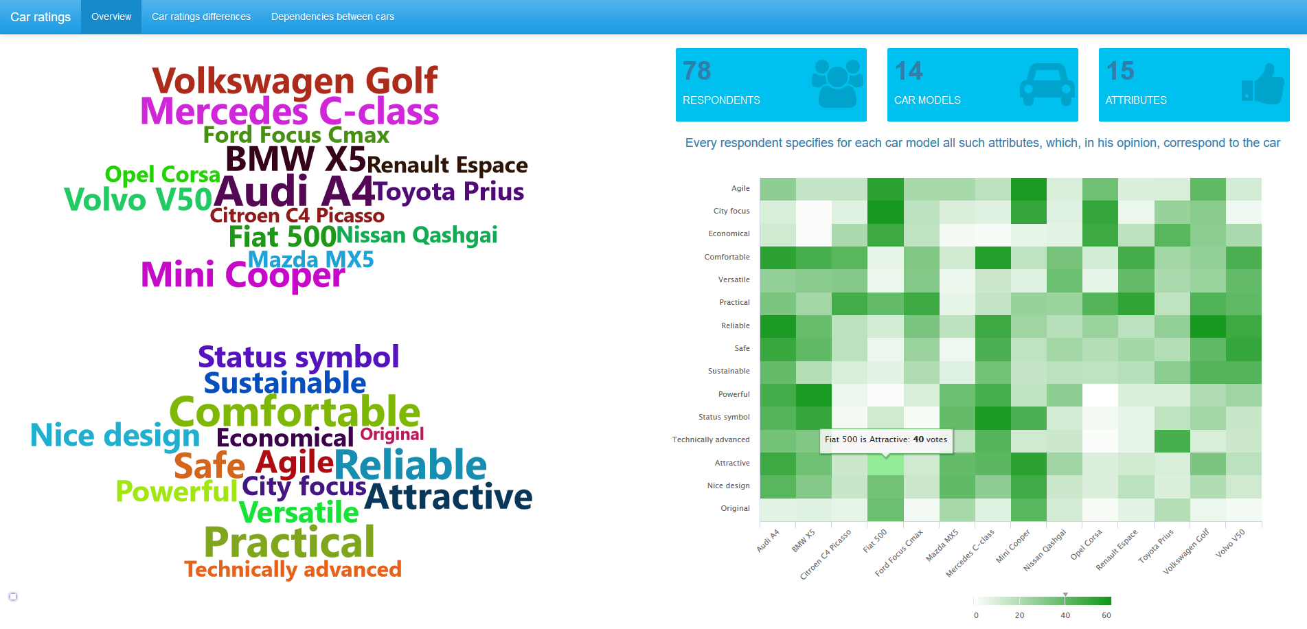
An overview of the data is given in the header picture, all pictures on a click are opened in full size. We see that 78 respondents took part in the survey. The research questionnaire found out opinions about 14 automobile brands. For each of them, respondents noted those characteristics (from the proposed list with 15 names) to which the car corresponds. The picture above shows that 40 respondents believe that the Fiat 500 is an attractive car.

Rating Comparison

To compare ratings on the characteristics between the two cars, the well-known McNemar test is used, more precisely, its variation of the McNemar mid-p test. This test analyzes paired observations. The mid-p correction allows you to work with small samples and is less conservative than an accurate binomial test. Details can be found, for example, in this article (Fagerland, Lydersen, and Laake 2013).

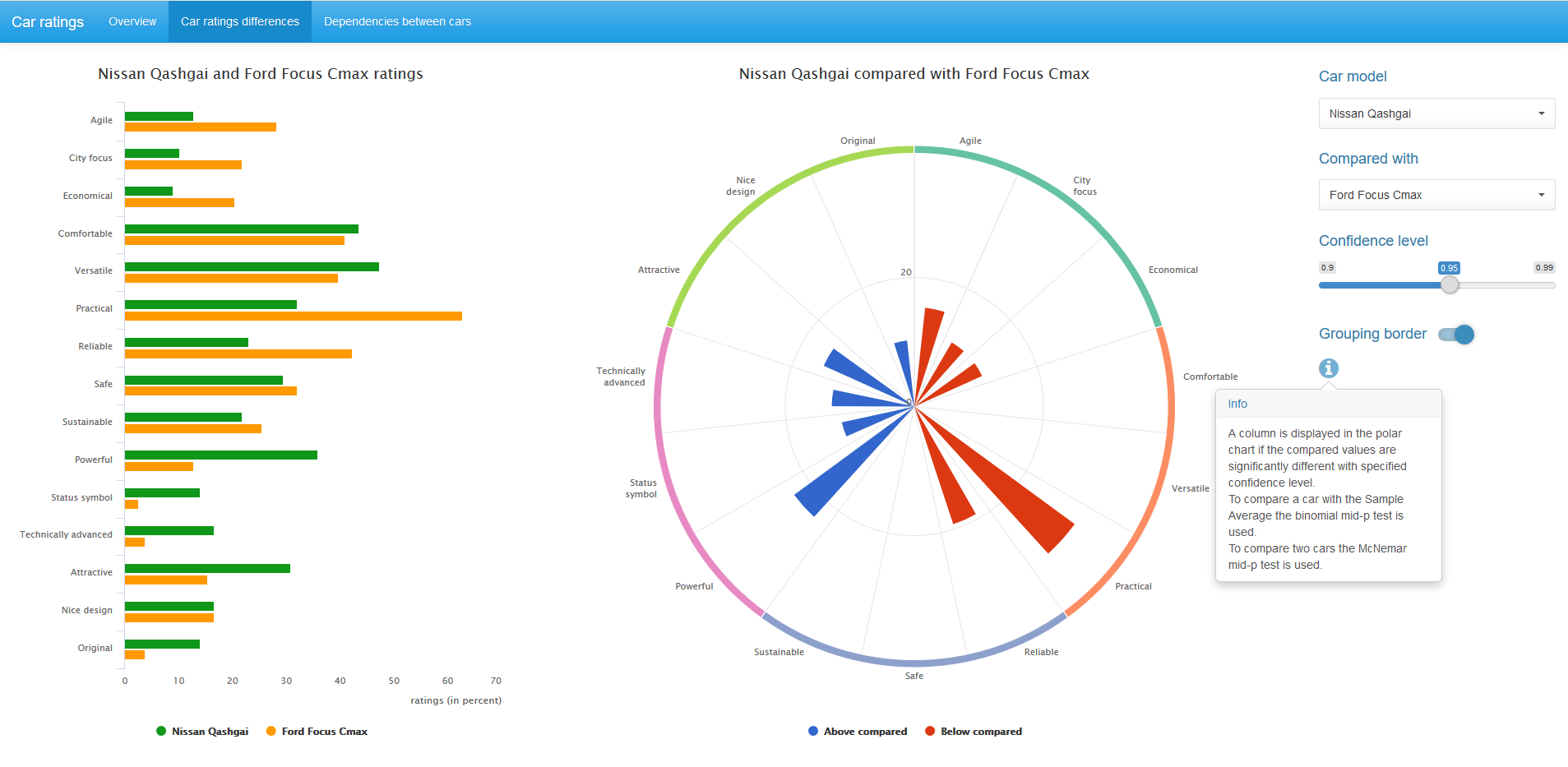
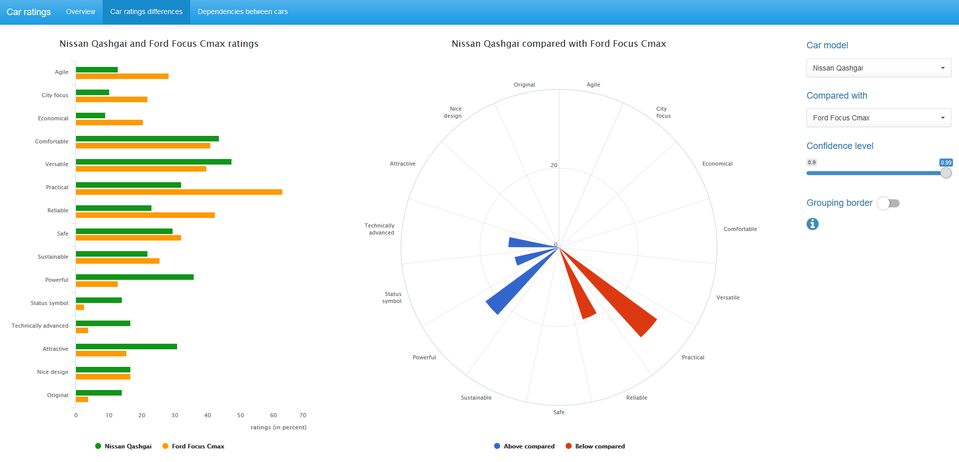
On the chart in the center, only statistically significant, for a given confidence level, difference in ratings between the pair of compared cars is displayed. Blue color corresponds to a higher rating value for the first car, red - for the second.

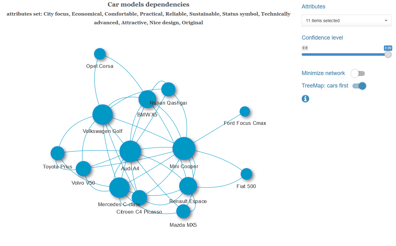
We can change the confidence level value and, if desired, remove the grouping border in the diagram.

You can also compare car ratings with average-selective ratings for all 14 cars. In this case, the binomial mid-p test is used.

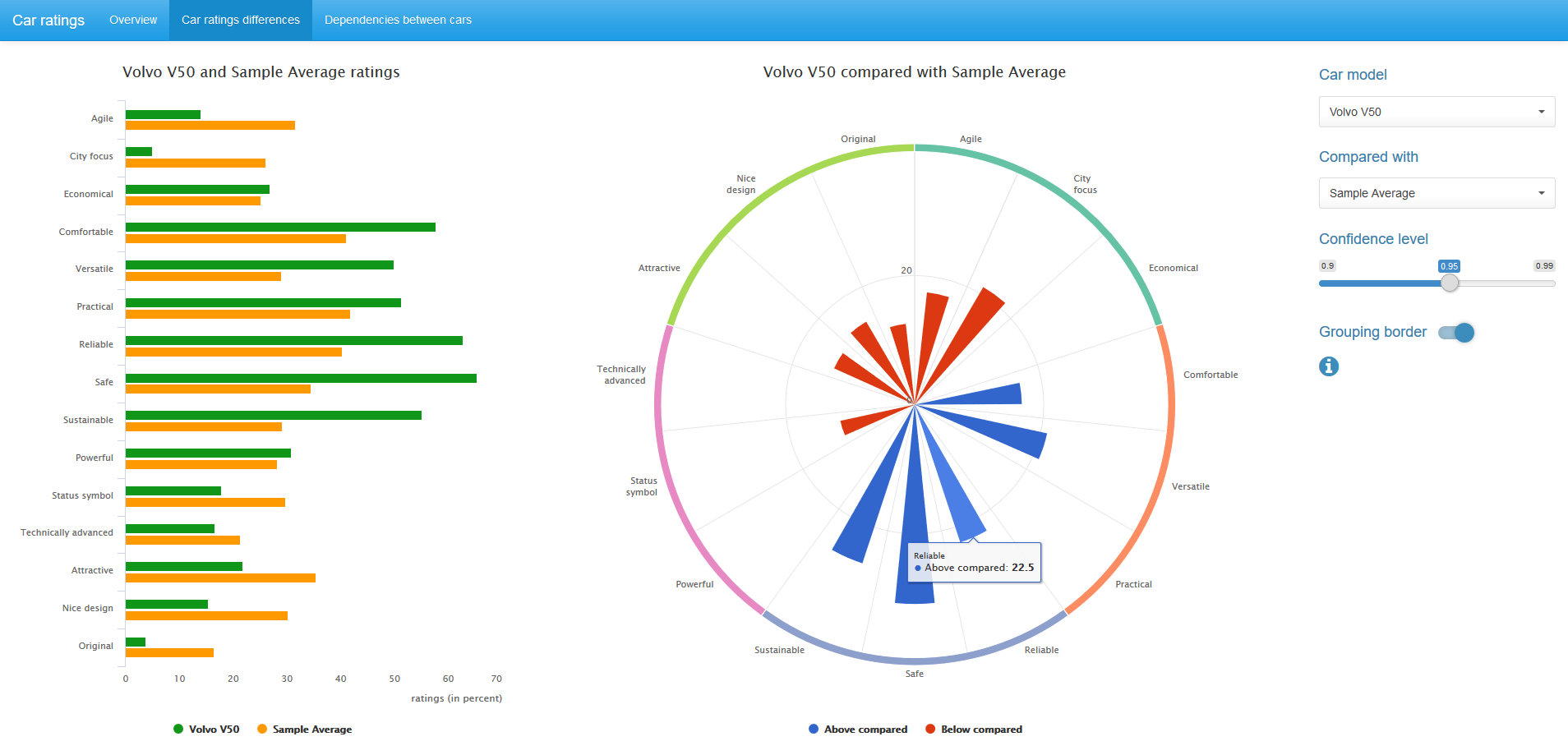
Both the McNemar mid-p test and the binomial mid-p test are available in the exact2x2 R package , but can be easily implemented using basic tools R.

Dependence between two multiple-response variables

The task is this: we have chosen any set of characteristics and an arbitrary pair of car models. Is it possible to state that the distribution of respondents' answers for these cars is independent? In other words, we have no reason to believe that there is any statistical relationship in the grading of these two brands in a given set of characteristics.

For example, consider an 8x8 table:

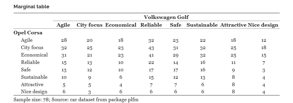
In it is the meaning of the cell, say Opel Corsa | Economical - Volkswagen Golf | Relible, equal to 41, means that exactly 41 respondents indicated that the Opel Corsa is an economical car and the Volkswagen Golf is reliable.

If both Opel Corsa and Volkswagen Golf were single-response variables, then this table would specify the joint distribution of these variables. Then we could apply the chi-square criterion to this table to check the independence of this pair of variables. But we have a completely different case and according to this table, for example, it is not even clear how many respondents believe that the Opel Corsa is an economical car.

Behind each cell of this marginal table sits a 2x2 table, which determines the distribution in a separate pair of selected characteristics. These 8 tables for the diagonal cells of the marginal table were just used in the McNemar tests for this pair of cars.

But this set of all 64 tables is not enough to specify the joint distribution of two multiple-response variables with 8 categories each. In general, this will require a table of size$$. So, the sum of 64 chi-square statistics found for 2x2 tables, due to the dependence of observations (not variables) in the input, is not a value$$distribution. Table information$$allow you to find the 2nd order Rao-Scott correction and apply it to the sum of these 64 chi-square values. Details and wording of the independence criterion can be found in the article (Bilder and Loughin 2004).

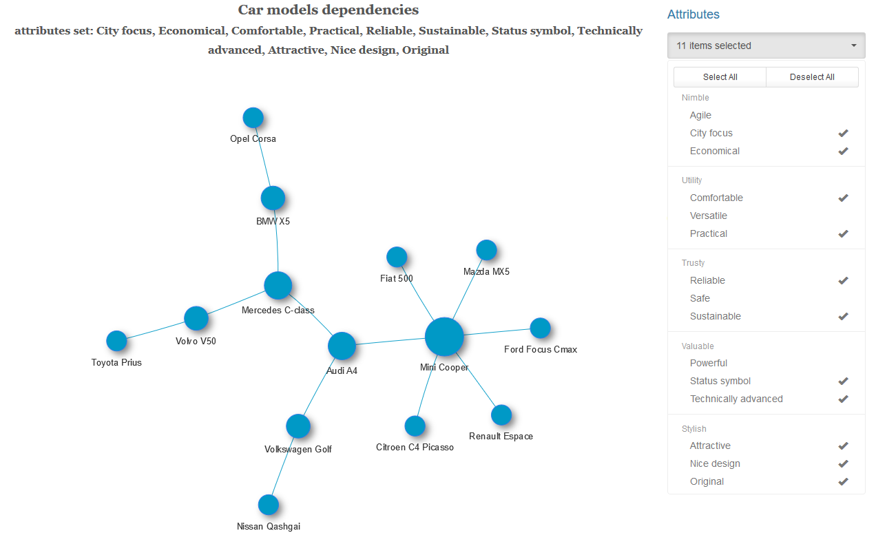
For each pair of cars with a given set of characteristics and at a selected level of significance, we test the hypothesis of independence of these variables. If the independence hypothesis is rejected, we connect this pair of cars with an edge with a weight equal to the p-value of the Rao-Scott statistics obtained. We get a weighted graph, to which we optionally apply the algorithm for finding the minimum spanning tree (for each connected component of the graph). That is, we leave the minimum possible number of the strongest bonds.

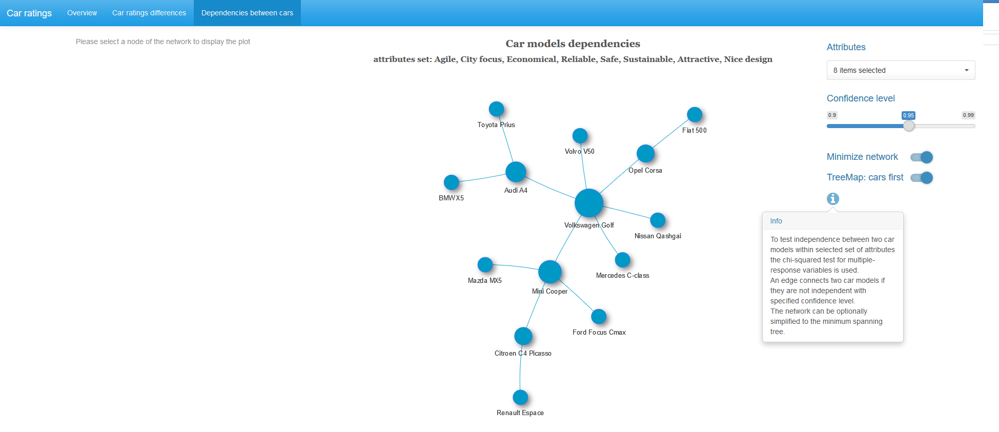
When you click on a picture, it will open in full size.
Almost half of the cars in the graph obtained have the strongest dependence with Volkswagen Golf.

If a graph vertex is selected, then in addition a treemap chi-square statistic of 2x2 tables with pairs of characteristics for adjacent vertices is displayed.

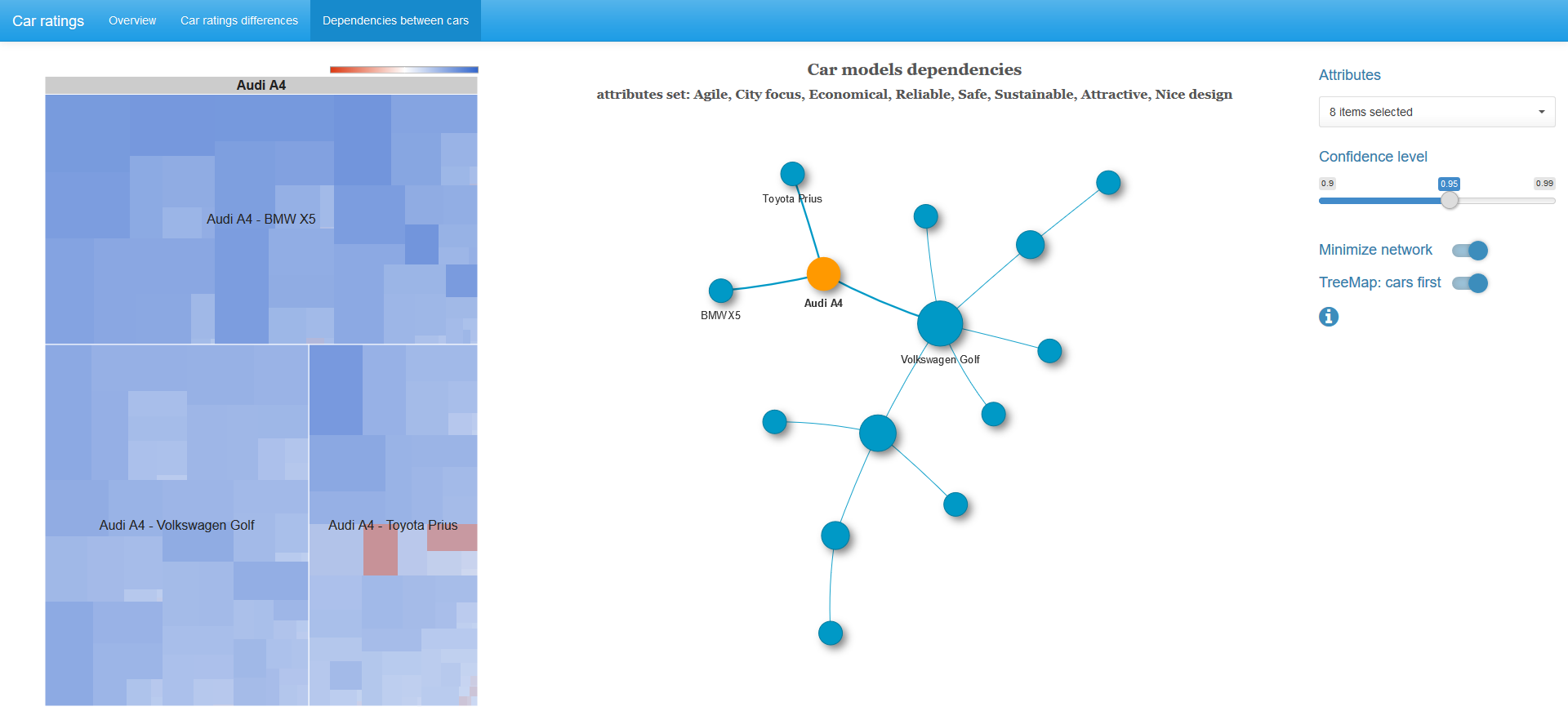
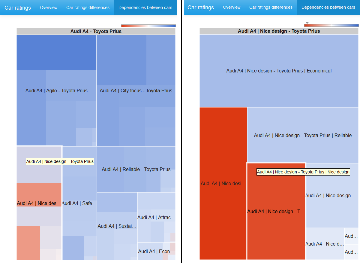
The size of the cell is proportional to the value of the chi-square statistic, the color is determined by the logarithm of the odds ratio: blue spectrum - positive values, white color - zero, red spectrum - negative values. The color scale is not symmetrical, that is, the left border in absolute value does not necessarily coincide with the right border of the scale.

Below are examples of a minimal spanning tree with a different set of characteristics and a graph with a complete set of links.

Computing and running the application

The approach proposed in (Bilder and Loughin 2004) is implemented in the MRCV R-package . However, for the 8x8 marginal table discussed above, the independence check function for these variables from this library returns an error: cannot allocate vector of size 32.0 Gb . The reason is that in the process of calculation, order matrices arise$$.

Был предложен подход, в котором реализация этого теста в R не требует столь большого объема памяти и является значительно более производительным. Для сравнения, вычисление полного графа с 14 вершинами и 7 характеристиками в пакете MRCV потребует более 30 минут. В улучшенной реализации это вычисление выполняется около 1 секунды. В этом pdf можно найти подробности этого метода вычислений. Исходный код и тесты производительности доступны на github.

Вы можете самостоятельно запустить это shiny приложение выполнив в R команды

library(shiny)
runGitHub("BrandsAnalysis", "e-chankov")

Предварительно убедитесь, что у вас установлены

#### shiny libraries
library(shiny)          # version 1.0.5
library(shinythemes)    # version 1.1.1
library(shinydashboard) # version 0.6.1
library(shinyBS)        # version 0.61
library(shinyWidgets)   # version 0.3.6
#### libraries for visualization
library(wordcloud2)     # version 0.2.0
library(highcharter)    # version 0.5.0
library(googleVis)      # version 0.6.2
library(visNetwork)     # version 2.0.1
library(RColorBrewer)   # version 1.1-2
#### data munging libraries
library(data.table)     # version 1.10.4
library(checkmate)      # version 1.8.4
library(Matrix)         # version 1.2-11 
library(igraph)         # version 1.1.2
library(stringi)        # version 1.1.5

Входные данные читаются из текстового файла. Приложение можно применить для анализа данных опросов о любых брендах со своим набором характеристик. Требования ко входным данным можно прочитать в описании приложения.

Литература

Bilder, C., and T. Loughin. 2004. “Testing for Marginal Independence Between Two Categorical Variables with Multiple Responses.” Biometrics 60 (1): 241–48. http://dx.doi.org/10.1111/j.0006-341X.2004.00147.x.

Fagerland, Morten W., Stian Lydersen, and Petter Laake. 2013. “The Mcnemar Test for Binary Matched-Pairs Data: Mid-P and Asymptotic Are Better Than Exact Conditional.” BMC Medical Research Methodology 13 (1): 91. https://doi.org/10.1186/1471-2288-13-91.

Van Gysel, E. 2011. “Perceptuele Analyse van Automodellen Met Probabilistische Feature Modellen.”
Master's thesis, Hogeschool-Universiteit Brussel.