Kaggle Mercedes and cross validation

Hello everyone, in this post I will talk about how I managed to take 11th place in the competition from Mercedes at kaggle , which can be described as a leader in terms of the number of participants and the epicity of shake-up. Here you can familiarize yourself with my solution , there is also a link to github, here you can see the presentation of my solution in Yandex .
This post will discuss how the student of the conservatory got into data science, became the winner of two consecutive kaggle-competitions, and how the methods of mathematical statistics help not to retrain on a public leaderboard.
I'll start by telling you a little about the problem and why I undertook to solve it. I must say that in data science I am a new person. About 7 years ago I graduated from the Physics Faculty of St. Petersburg State University and since then I have been engaged in getting a musical education. The idea to stretch my brain a bit and return to technical tasks first visited me about two years ago, at that time I already worked in the Moscow Philharmonic Orchestra and was in my 3rd year at the Conservatory. I began with the fact that, armed with a book by Straustrup, I began to learn C ++. Further, of course, there were various online courses, and about a year ago I began to incline to the idea that Data Science is perhaps exactly what I would like to do in IT. My “education” in Data Science is a course from Yandex and HSE on a cursor , several courses fromMIPT specializations in the course and, of course, constant self-development in competitions.
I got my first kaggle medal in the competition from Sberbank - I took 13 out of 3000+ places there, here is the decision of Sberbank with reference to github. And right after that I decided to fit into the competition from Mercedes, before which 10 days remained. It was a very difficult 10 days of my vacation, but, firstly, I discovered a lot of new things, and secondly, I got one more gold medal in the end. And in this post I would like to share what I learned while solving this problem.
Formulation of the problem
There is some kind of installation at the Mercedes factory that is testing new cars. Testing time varies widely enough - approximately from 50 to 250 seconds. We are invited to predict this time on more than 300 different grounds. All signs are anonymized, but the organizers revealed their common meaning. There were 8 categorical signs (they took values of the form A, XV, FD, B, ...), and these were the characteristics of the car. Most of the signs took the values 0 or 1 and were characteristics of the tests that were carried out for each particular machine.
Now that the overall plan is clear, it's time to move on to the details. Here I would like to make a reservation right away that I will not discuss the subtleties of ensemble algorithms or some non-trivial tricks of gradient boosting later in the text. This will mainly focus on how to validate so as not to get upset when opening a private leaderboard. If we discard all the artistic details, we have the usual task of regression on anonymized features. The peculiarity of this competition consisted of a small (by kaggle standards) dataset (train and test of approximately 4000 objects) and a very noisy target (box spot target below).

From boxplot, it becomes obvious that we will encounter difficulties in validating. It can be assumed that cross-validation awaits us with a hefty spread of metrics on folds. And to add fuel to the fire, I’ll clarify that the competition metric is the determination coefficient (R2), which, as you know, is very sensitive to emissions.
The task attracted so many participants primarily because the base line is written in several lines. Let's make such a baseline and look at the results of cross-validation:
import xgboost as xgb
from sklearn.model_selection import cross_val_score
import pandas as pd
import numpy as np
data = pd.read_csv('train.csv')
y_train = data['y']
X_train = data.drop('y', axis=1).select_dtypes(include=[np.number])
cross_val_score(estimator=xgb.XGBRegressor(), X=X_train, y=y_train,
                cv=5, scoring='r2')
The conclusion will be something like this:
[ 0.37630003, 0.43968909, 0.5886552 , 0.54800137, 0.55752035]The standard deviation for folds is so great that comparing the means loses its meaning (in the vast majority of cases, the means will differ by less than the standard deviation).
Everything that comes next consists of two parts. The first part is simple and enjoyable, which aroused keen interest in training at Yandex. In it, I will explain why a large std (Standard Deviation) is not a hindrance to cross-validation and show a beautiful and uncomplicated approach that eliminates the impact of this std. The second part is more complex, but, in my opinion, much more important. In it I will talk about why this is not a panacea, how cross-validation can lead us astray, what makes sense to expect from cross-validation and how to relate to it. So let's go.
Comparison of models on noisy data
Why do we need cross-validation at all? When we solve the problem, we try a huge number of different models and want to find the best or the best. Thus, we need a way to compare two models and reliably choose a winner from this pair. This is exactly what we are asking for cross-validation for help from. I will make a reservation that by model I understand not just some kind of machine learning algorithm, but the entire pipeline, which includes data preprocessing, selection of features, creation of new features, selection of an algorithm and its hyperparameters. Any of these steps is essentially a hyperparameter of our model, and we want to find the best hyperparameters for our task. And for this it is necessary to be able to compare two different models. Let's try to solve this problem.
Let me remind you that the value of the loss function for the cross-validation folds in the Mercedes problem is catastrophically unstable. Therefore, simply comparing the average speed of the two models in cross-validation, we cannot draw any conclusions (the differences will be within the margin of error). I used this approach:
1. We will make not one split into 5 folds, but 10. Now we have 50 folds, but the fold size remains the same. In the scores array, we get 50 scores on fifty test folds:
import numpy as np
from sklearn.model_selection import KFold, cross_val_score
scores = np.array([])
for i in range(10):
    fold = KFold(n_splits=5, shuffle=True, random_state=i)
    scores_on_this_split = cross_val_score(
            estimator=xgb.XGBRegressor(), X=X_train, y=y_train,
            cv=fold, scoring='r2')
    scores = np.append(scores, scores_on_this_split)
2. We will compare not the average speed of the models, but how much each model is better or worse than the other on the corresponding fold. Or, what is the same, we will compare with zero the average of pairwise differences of the results of two models on the corresponding folds .
Further, I formalize the second point a little, but now I need to understand that cheers, we no longer depend on the fact that, say, we have an outlayer in the first fold, and the speed there is always very low. Now the speed on the first fold is not averaged with the rest, it is compared exclusively with the speed on the same fold of the second model. Accordingly, it no longer bothers us that the first fold is always worse than the second, because we compare not the average speed, but the speed on each fold, and only then average it.
Now let's move on to assessing statistical significance. We want to answer the question: are the scores of our two models significantly different on our 50 test folds. The scores of our models are related samples, and I propose using a statistical criterion specifically designed for such cases. This is student t-test for related samples. I will not overwhelm the post with arguments that the hypothesis of normality is fulfilled in our case with sufficient accuracy, and the Student criterion is applicable - I dwell on this at a training in Yandex, you can watch the recording if you wish. Now I will immediately go to the practical part.
Statistics of the t-criterion is as follows:

Where
 - lists of metric values for test folds for the first and second models, respectively, S is the variance of pairwise differences, n is the number of folds. Here I want to make a reservation that I will not be able to describe the procedure for testing statistical hypotheses and the theory that is behind this. Not because it is difficult to understand, but simply because, it seems to me, the post is not really about that. And also because it’s difficult enough to explain and, having made this post two screens longer, I’m still unlikely to make these things clearer to people for whom they are new. In the first two weeks of this course, the topic of testing statistical hypotheses is comprehensively disclosed, I highly recommend: https://www.coursera.org/learn/stats-for-data-analysis/home/welcome .
So, our null hypothesis is that both models give the same results. In this case, the t-statistics is distributed according to Student with a mathematical expectation of 0. Accordingly, the more it deviates from 0, the less is the probability that the null hypothesis is fulfilled, and the averages in the numerator of the fraction do not coincide purely by chance. Note the denominator: S is the variance of pairwise differences . That is, we are not at all interested in the variance of the scores on the folds for each model individually (i.e., the variance
 and
and  ), we are only interested in how "stably" one model is better or worse than another. It is for this that S is responsible, being in the denominator.
 The criterion of interest to us is implemented in the scipy library in the stats module, this is the ttest_rel function. The function accepts two lists (or arrays) of metrics on the test folds as an input, and returns the value of t-statistics and p-value for a two-way alternative. The larger the t-statistics modulo, and the smaller the p-value, the more significant the differences. The most common practice is to consider that differences are significant if p-value <0.05. Let's see how it works in practice:
import xgboost as xgb
from sklearn.model_selection import cross_val_score, KFold
import pandas as pd
import numpy as np
from scipy.stats import ttest_rel
data = pd.read_csv('./input/train.csv')
y_train = data['y']
X_train = data.drop('y', axis=1).select_dtypes(include=[np.number])
scores_100_trees = np.array([])
scores_110_trees = np.array([])
for i in range(10):
    fold = KFold(n_splits=5, shuffle=True, random_state=i)
    scores_100_trees_on_this_split = cross_val_score(
                                             estimator=xgb.XGBRegressor(
                                                        n_estimators=100),
                                             X=X_train, y=y_train,
                                             cv=fold, scoring='r2')
    scores_100_trees = np.append(scores_100_trees,
                                 scores_100_trees_on_this_split)
    scores_110_trees_on_this_split = cross_val_score(
                                            estimator=xgb.XGBRegressor(
                                                        n_estimators=110),
                                            X=X_train, y=y_train,
                                            cv=fold, scoring='r2')
    scores_110_trees = np.append(scores_110_trees,
                                 scores_110_trees_on_this_split)
ttest_rel(scores_100_trees, scores_110_trees)
We get the following:
Ttest_relResult(statistic=5.9592780076048273, pvalue=2.7039720009616195e-07)Statistics are positive, which means that the numerator of the fraction is positive and, accordingly, the average
more than average . Recall that we maximize the target metric R2 and understand that the first algorithm is better, that is, 110 trees on this data lose 100. The P-value is much less than 0.05, so we boldly reject the null hypothesis, claiming that the models are significantly different. Try to calculate mean () and std () for scores_100_trees and scores_110_trees and you will see that simply comparing the averages does not work here (the differences will be of the order of std). Meanwhile, the models are different, and they differ very much, and the Student t-test for related samples helped us show this.I would end the first part on this, but for some reason I already imagine how many readers, armed with this knowledge, will make a tremendous GridSearch, do thousands of scores_xxx arrays, do thousands of t-tests, compare it all with the base line, and choose an algorithm with the largest modulus of negative t-statistics (or positive, depending on the order of the arguments ttest_rel). Friends, colleagues, wait, do not do this. GridSearch is a very insidious thing. Let's remember that our t-statistics are distributed by student. This means that, firstly, this is a random variable, and secondly, even assuming no differences whatsoever, it can take values from minus infinity to infinity. Think about it: from minus infinity to infinity for models, which will actually give almost the same speed on new data! On the other hand, the larger the value of t-statistics modulo, the less likely it is to get it randomly. That is, for example, the probability that we will get something more than 3 in absolute value is less than 0.5%. But you did GridSearch, checked several thousand different models. Obviously, even if they didn’t differ at all, at least once you are likely to overcome this three. And accept the wrong hypothesis. overcome this three. And accept the wrong hypothesis. overcome this three. And accept the wrong hypothesis.
In statistics, this is called multiple checking, and there are different methods for dealing with errors in this same multiple checking. I propose to use the simplest of them - to test fewer hypotheses and do it very meaningfully. Now I will explain how I see this in practice.
Let's go back to our xgboost and try to optimize the number of trees. First, I urge you to optimize hyperparameters strictly one at a time. Let us have a base line - 100 trees. Let's see what happens with t-statistics with a smooth decrease in the number of trees to 50:
%pylab inline
t_stats = []
n_trees = []
for j in range(50, 100):
    current_score = np.array([])
    for i in range(10):
        fold = KFold(n_splits=5, shuffle=True, random_state=i)
        scores_on_this_split = cross_val_score(
                                      estimator=xgb.XGBRegressor(
                                                   n_estimators=j),
                                      X=X_train, y=y_train,
                                      cv=fold, scoring='r2')
        current_score = np.append(current_score,
                                  scores_on_this_split)
    t_stat, p_value = ttest_rel(current_score, scores_100_trees)
    t_stats.append(t_stat)
    n_trees.append(j)
plt.plot(n_trees, t_stats)
plt.xlabel('n_estimators')
plt.ylabel('t-statistic')
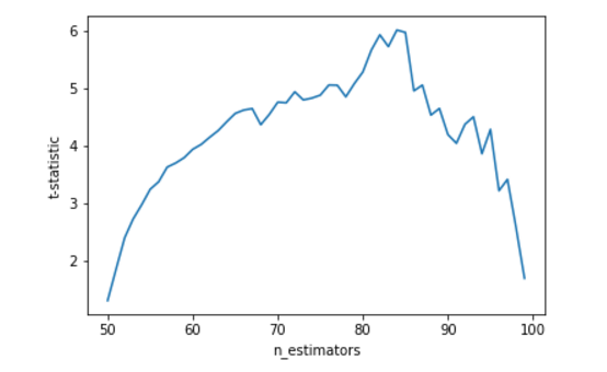
What we see on the chart is a good situation. When we have about 50 trees, the responses of the model are not much different from the baseline with a hundred trees. With an increase in the number of trees, the differences increase, the algorithm begins to predict better: somewhere around 85 we have an optimum, and then the t-statistics fall, that is, the algorithm approaches our base line. Looking at the graph, it becomes obvious that the optimal number of trees is approximately 83. But it is quite possible to take 81, 82, 83, 84, 85 and average. This kind of averaging makes it possible, almost for free in the sense of our efforts, to improve the generalizing ability and the final speed; I often use this technique. I hope that from all these considerations it becomes clear that on such graphs we are interested not just in the global optimum, but in the optimum, to which the function smoothly strives and from which it smoothly leaves. With a sufficiently large number of points on the graph, we can well get random bursts, which may be more than the optimum of interest to us. But we differ from GridSearch in that we will take not just a point with the maximum (minimum) value of t-statistics, but we will approach this a little more reasonably.
In order to be able to look at such graphs, I urge you to optimize hyperparameters in turn. In some cases, it may be justified to switch to a 3-dimensional scatter-plot, on which you can monitor the metric depending on two hyperparameters.
Unfortunately, I can’t summarize the first part with the plan of the view, first do it like this, then like that, since setting hyperparameters for cross-validation is a very delicate matter and requires constant analysis. The only thing I definitely insist on: never try to get into the top ten - it's impossible. The fact that 148 trees are better than 149 in cross-validation does not mean at all that the test will be the same. Not sure - average, because averaging is one of the very few things that the model: a) will definitely not ruin, b) is likely to improve. And be careful with GridSearch - this algorithm is very good at creating the appearance of optimizing hyperparameters. At least for those hyperparameters that you consider important in this task, you must manually verify that you have found a really optimal value,
The danger of retraining on emissions
In the second part of my post, I will discuss what cross-validation is in principle, how and how it can help us, and what it cannot. The background is as follows: applying the validation that I talked about in the first part, I started to improve the model: tweak something somewhere, select features, add new ones, generally do what we always do when solving kaggle. I approached the testing of statistical hypotheses very conservatively, I tried to test them as little as possible and as reasonably as possible. Quickly enough, I came to the conclusion that the average R2 in cross-validation was approximately 0.58. As we know today, the best private leaderboard speed is 0.5556. But then I didn’t know this, and on the public leaderboard the top was already 0.63+, although it was clear it’s absolutely useless to look at other people's publics (leaderboard probing in this competition was an unprecedented scale). A cold shower happened when I made a submission the best, in my opinion, model and got 0.54 on the public, despite the fact that the base line gave 0.55. It became obvious that something was wrong here.
At this point, I would like to dwell a little more. If, for example, it was not kaggle, but work, I would have every chance of sending such a model to production (at least try to do it). It would seem that this? I have such a cunning cross-validation, I carefully selected all the parameters and got a high speed, what could be the questions? But you need to understand, and always remember about what I forgot then - cross-validation, in principle, cannot evaluate the performance of a model on new data. Just in case, I’ll explain that by the word performance I mean the quality of the model’s work in terms of the chosen metric. You do cross-validation over and over again, choosing only those models that work best on test folds. Not on some test folds, but on completely specific and identical test folds. And even if you, say, change random_state from Kfold periodically, thereby making folds different, they are all the same, ultimately, collected from the objects of your training set. And, selecting hyperparameters, you train the algorithm exactly on these objects. If the data is good, and we did everything carefully, then this may lead to the algorithm working slightly better on new objects, but in general, you should not expect the same performance. And in the case when the data is quite noisy, there is a risk of encountering a situation that I encountered and which I will discuss until the end of the post. then this can lead to the fact that the algorithm will work a little better on new objects, but in general, you should not expect the same performance. And in the case when the data is quite noisy, there is a risk of encountering a situation that I encountered and which I will discuss until the end of the post. then this can lead to the fact that the algorithm will work a little better on new objects, but in general, you should not expect the same performance. And in the case when the data is quite noisy, there is a risk of encountering a situation that I encountered and which I will discuss until the end of the post.
For myself, I realized that it is absolutely necessary to have a delayed selection in any task. I would suggest doing this: get the task - immediately make a delayed selection and throw it out of the train. We calculated the result of the base line on this sample. Then you can improve the model for a long time and persistently, and finally, when the best model is already ready, it's time to see the speed on the delayed selection. In the case of kaggle, the public leaderboard can play the role of delayed sampling. But it is important to remember that the more often we look at the speed of the delayed sample, the worse it estimates the performance of the model on new data.
Going back to Mercedes. Having received a public speed lower than my base line, I realized that I was retrained. Now I will demonstrate how retraining occurs with the seemingly correct approach to the selection of hyperparameters. For clarity, we will have only one feature. Let the true dependence be the sine, add normal noise and add normal emissions (15% less objects, 4% more emissions):
import numpy as np
import seaborn as sns
import numpy as np
%pylab inline
np.random.seed(3)
X = 8 * 3.1415 * np.random.random_sample(size=2000)
y = np.sin(X) + np.random.normal(size=X.size, scale=0.3)
outliers_1 = np.random.randint(low=0, high=X.shape[0], size=int(X.shape[0] * 0.15))
y[outliers_1] += np.random.normal(size=outliers_1.size, scale=1)
outliers_2 = np.random.randint(low=0, high=X.shape[0], size=int(X.shape[0] * 0.04))
y[outliers_2] += np.random.normal(size=outliers_2.size, scale=3)
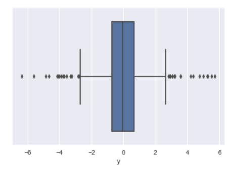
sns.boxplot(y)
plt.show()
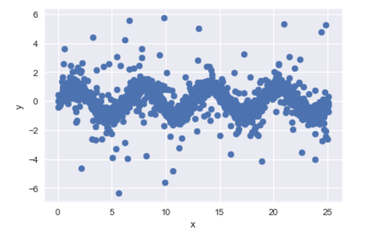
plt.scatter(x=X, y=y)
plt.show()
Boxplot is somewhat similar to what we saw for the target in the task from Mercedes, but emissions are present on both sides.
Let the first thousand objects be our training sample, the second a test one. Let's calculate the baseline speed for cross-validation:
import xgboost as xgb
from sklearn.model_selection import cross_val_score,KFold
from scipy.stats import ttest_rel
X_train = X[:X.shape[0]/2].reshape(-1,1)
y_train = y[:X.shape[0]/2]
X_test = X[X.shape[0]/2:].reshape(-1,1)
y_test = y[X.shape[0]/2:]
base_scores_train = np.array([])
for i in range(10):
    fold = KFold(n_splits=5, shuffle=True, random_state=i)
    scores_on_this_split = cross_val_score(
                                     estimator=xgb.XGBRegressor(
                                             min_child_weight=2),
                                     X=X_train, y=y_train,
                                     cv=fold, scoring='r2')
    base_scores_train = np.append(base_scores_train,
                                  scores_on_this_split)
Now, just as we did in the first part, compare with a base line model with fewer trees and look at the dependence of t-statistics on n_estimators:
t_stats_train = []
for j in range(30, 100):
scores_train = np.array([])
for i in range(10):
fold = KFold(n_splits=5, shuffle=True, random_state=i)
scores_on_this_split = cross_val_score(
estimator=xgb.XGBRegressor(
n_estimators=j, min_child_weight=2),
X=X_train, y=y_train, cv=fold, scoring='r2')
scores_train = np.append(scores_train,
scores_on_this_split)
t_stat,p_value = ttest_rel(scores_train, base_scores_train)
t_stats_train.append(t_stat)
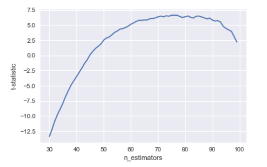
plt.plot(range(30, 100), t_stats_train)
plt.xlabel('n_estimators')
plt.ylabel('t-statistic')
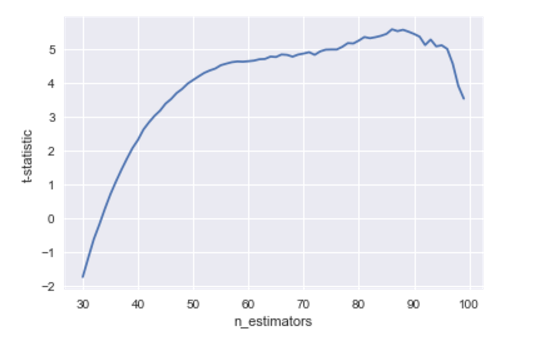
We get a very beautiful graph, from which we conclude that it is optimal to take about 85 trees:
But let's see how these algorithms behave on the new data:
est_base = xgb.XGBRegressor(min_child_weight=2)
est_base.fit(X_train, y_train)
base_scores_test = r2_score(y_test, est_base.predict(X_test))
scores_test = []
for i in range(30,101):
    est = xgb.XGBRegressor(n_estimators=i, min_child_weight=2)
    est.fit(X_train,y_train)
    scores_test.append(r2_score(y_test, est.predict(X_test)))
plt.plot(range(30, 101), scores_test)
plt.xlabel('n_estimators')
plt.ylabel('r2_score_test')
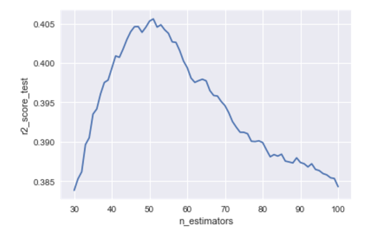
We are surprised to find that 85 is far from the optimal number of trees for our dataset. Emissions are of course to blame, and it is in this situation, as it seems to me, that I got into a Mercedes contest. If you experiment with this code, you will see that it is not at all necessary that the optimum on the train is to the right of the optimum on the test, but quite often their x-coordinate will not coincide.
To assess how strongly emissions affect the speed, I suggest tormenting this line:
from sklearn.metrics import r2_score
r2_score(
    [1,   2,    3,   4,   5,   11],
    [1.1, 1.96, 3.1, 4.5, 4.8, 5.3]
)
Please note that if, for example, instead of 1.1, we write 1.0 in the second array, the speed will change in the fourth character. Now let's try to get 0.1 closer to our outlier - we’ll replace 5.3 with 5.4. The speed changes immediately by 0.015, that is, about 100 times stronger than if we improved the prediction of the “normal” value by the same amount. Thus, the speed is mainly determined not by how accurately we predict "normal" values, but by which model accidentally turned out to be slightly better on emissions. And it becomes clear that when selecting signs and tuning hyperparameters, we involuntarily select those models that guess emissions better on test folds, rather than those that better predict the bulk of objects. This is simply because out-guessing models get a higher rate,
In most tasks, I believe, emissions cannot be predicted. This must be verified, and if so, openly admit it. And since we cannot predict them, let's not take them into account when comparing models. Indeed, if any of our models is equally bad at predicting outliers on new data, then what's the point of evaluating outlook predictions on cross-validations? There are two strategies for behavior in such situations:
1. Let's remove all outliers from the training set and only after that we will train and validate the models. We will talk about exactly how to remove emissions a little later, while we believe that somehow we can do it. This strategy is really very strong, the winner of the Sberbank Russian Housing Market contest, Evgeny Pateha, was validated exactly like this: youtu.be/Eo4WMlcT7uo ,www.kaggle.com/c/sberbank-russian-housing-market/discussion/35684 . The only problem with this method is that often throwing outlayers biases the average prediction, and we are forced to somehow compensate for this bias.
2. We will not remove anything from the training set, but during validation (when calculating the metric value on test folds) we will not take into account outliers. I used just such a scheme. You can find my implementation of such cross-validation in this repository , a function called cross_validation_score_statement is defined in the file cross_val_custom.py. Once again, all the way up to calling the fit method (and including it) we do it without throwing anything, then we make predict on test folds, but we only consider the metric on objects that are not outliers.
As I said, having received a very low speed on public, I realized that I was retraining. When I began to validate without outsourcers, this retraining immediately became obvious. It turned out that I too aggressively selected signs that too many trees were growing for my xgboosts. It turned out to be very easy to fix everything, I spent about an hour trying to find a new optimum in the space of hyperparameters, and sabotaged the result. The transition to validation without outsourcers made the decision 11th place out of the 3000+ solution at the privet.
We show how it works on our toy dataset. First, you need to decide who to consider as an outlayer. I considered outlays objects on which the base line is mistaken most of all (the out-of-fold prediction error is greater than some threshold). The threshold is selected based on how many percent of the training sample you want to declare as outsiders.
from sklearn.model_selection import cross_val_predict
base_estimator = xgb.XGBRegressor(min_child_weight=2)
pred_train = cross_val_predict(estimator=base_estimator, X=X_train, y=y_train, cv=5)
abs_train_error = np.absolute(y_train - pred_train)
outlier_mask = (abs_train_error > 1.5)
print 'Outliers fraction in train = ',\
float(y_train[outlier_mask].shape[0]) / y_train.shape[0]
We get:
Outliers fraction in train = 0.045That is, 4.5% of objects are declared emissions. Now let's calculate the cross validation scores for the base line, and then we will change the number of trees. Only now emissions will not be taken into account when calculating the speed.
# import cross_val_custom from
# https://github.com/Danila89/cross_validation_custom
from cross_val_custom import cross_validation_score_statement
from sklearn.metrics import r2_score
base_scores_train_v2 = np.array([])
for i in range(10):
    scores_on_this_split = cross_validation_score_statement(
                                        estimator=xgb.XGBRegressor(
                                           min_child_weight=2),
                                        X=pd.DataFrame(X_train),
                                        y=pd.Series(y_train),
                                        scoring=r2_score, n_splits=5,
                                        random_state=i,
                                        statement=~outlier_mask)
    base_scores_train_v2 = np.append(base_scores_train_v2,
                                     scores_on_this_split)
t_stats_train_v2 = []
for j in range(30, 100):
    scores_train_v2 = np.array([])
    for i in range(10):
        fold = KFold(n_splits=5, shuffle=True, random_state=i)
        scores_on_this_split = cross_validation_score_statement(
                                        estimator=xgb.XGBRegressor(
                                            n_estimators=j,
                                            min_child_weight=2),
                                        X=pd.DataFrame(X_train),
                                        y=pd.Series(y_train),
                                        scoring=r2_score, n_splits=5,
                                        random_state=i,
                                        statement=~outlier_mask)
        scores_train_v2 = np.append(scores_train_v2,
                                    scores_on_this_split)
    t_stat,p_value = ttest_rel(scores_train_v2, base_scores_train_v2)
    t_stats_train_v2.append(t_stat)
plt.plot(range(30,100), t_stats_train_v2)
plt.xlabel('n_estimators')
plt.ylabel('t-statistic')
We get the following graph:
It can be seen that, unfortunately, this is not a silver bullet, and the optimum is still not located on 50 trees, as we would like. But this is no longer 85 as it was before, and the extremum is not so obvious, which suggests that it makes sense to average from 60 to 95 over the number of trees. And having done this, it is quite possible to get a result comparable to that we would get if we knew that we really need to take 50.
And the last thing I want to show is how the predictions of our boost actually change with an increase in the number of trees, since in the one-dimensional case this can be done. For different n_estimators, I will build the predictions of the algorithm and glue this into a gif:
X_plot = np.linspace(0,8 * 3.1415, num=2000)
est = xgb.XGBRegressor(n_estimators=70, min_child_weight=2)
est.fit(X_train, y_train)
plt.plot(X_plot, est.predict(X_plot.reshape(-1, 1)))
plt.xlabel('X')
plt.ylabel('Prediction')
We see how much the outlayers prevent our model from working. We also see that after about n_estimators = 60, the model actually stops approaching the original function and only deals with retraining on outliers from the training set. Recall that on our “new” data, 50 trees show themselves best. And on animations with n_estimators = 60, 70, 80, t-statistics on cross-validation continues to increase, and it grows precisely due to a successful hit in outlayers. When I made this animation, the idea of training models on a clean dataset began to seem even more attractive to me. A lot more can be said by looking at this gif, but I dare not hold you back anymore.
I really hope that you do not regret the