Introduction

Many engineers in the field of electromagnetic modeling often have questions about the further processing and use of the simulation results of the problem in other environments, or, conversely, the transfer of parameters from one medium to another. It would seem that there is no problem exporting the results to a form understandable by another program and using them, or entering data manually. However, tasks often arise that require performing this sequence of actions N times and the performance of these actions tends to zero. If you are interested in the topic indicated in the title, then please, under cat.

Current data processing trends have led radio engineers to use the powerful Mathworks Matlab tool everywhere to achieve their goals.. This package allows you to solve the problems of digital signal processing, FPGA modeling and communication systems in general, the design of radar models and much more. All this makes Matlab an indispensable assistant for almost any radio engineer.

Specialists in high-precision electrodynamic modeling often operate with other specific software packages, one of which is CST Microwave Studio . There are many articles on this product on the Eurointech website . Therefore, there is no need to dispute its leading aspects.

The author recently faced the task of simultaneously using the packages mentioned above. In this article, I would like to reflect a possible way to solve this problem, as well as a range of similar tasks.

Strategy

In the general case, it was necessary to simulate a project in Microwave Studio in the frequency range specified by a certain function performed in Matlab, and then use the results of modeling transmission coefficients S _ij in other calculations.

The method of manual data input and output fell immediately, since the described sequence of actions had to be performed from 1 to several thousand times.

It was decided to try to establish control of Microwave Studio simulation parameters directly from Matlab functions. An analysis of the available CST and Matlab help, as well as Internet resources, showed that both programs support the use of the ActiveX framework.
Activex- A framework for defining software components suitable for use from programs written in different programming languages. Software may be assembled from one or more of these components in order to utilize their functionality.

This technology was first introduced in 1996 by Microsoft as a development of the Component Object Model (COM) and Object Linking and Embedding (OLE) technologies and now it is widely used in Microsoft Windows operating systems, although the technology itself is not tied to the operating system.

From the description of CST Studio it follows that any of its components can act as a managed OLE server. OLE is a technology for linking and embedding objects in other documents and objects, developed by Microsoft. Thus, here it is a Microsoft Windows solution, Matlab, CST Microwave Studio + OLE technology.

Now you need to figure out how to implement all this in Matlab.

Basic functions for managing CST from Matlab

From [1], several basic functions necessary for working with the ActiveX interface can be distinguished:

actxserver

- create a local or remote server;

invoke

- call the method for the ActiveX object.

Simply put, the essence of the actxserver command is to initialize (open) a program that acts as a managed program, invoke - to refer to certain sections of a managed program.

Example:

сst = actxserver('CSTStudio.Application')

- the command binds the CSTStudio.Application object managed by OLE to the variable “cst ”. In this case, the name " CSTStudio.Application " is a unique name in the ActiveX environment, allowing you to understand which program we want to access.

mws = invoke(cst , 'NewMWS')

- allows you to navigate between the main program menus, in this case sends a command to the “ cst ” variable associated with the CST Studio application to create a new empty project file;

invoke(mws, 'OpenFile', '<Путь к файлу>')

- sends a command to open a specific file located at <File Path> in the newly created empty tab, which is associated with the variable "mws";

solver = invoke(mws, ‘Solver’)

–– this command assigns the solver variable to the solver tab in the project tab associated with the “ mws ” variable of Microwave Studio;

invoke(solver, 'start')

- this team, turning to CST Studio for an open project, will go into the solver tab and start calculating the model.

If you turn to the Workspace tab in Matlab and see the values ​​of the (Value) variables: cst , mws , solver , you will notice the following:

• The cst variable has a value of <1x1 COM.cststudio_application> . This means that the cst variable is connected to the main Microwave Studio window, and you can create files in it, close it, etc. If the file is created using the invoke function (cst, 'NewMWS') , then closing is performed by the command
  
  

  invoke(cst, 'quit')

  
  
• The mws variable has a value of <1x1 Interface.cststudio_application.NewMWS> . This means that the mws variable is associated with a specific project tab in the main CST window. In the project tab, you can open finished projects, save and close them, and also go to the tabs for working on the project.
  
  Examples of commands:
  
  

  invoke(mws, 'save')

  - save the current project;
  
  

  invoke(mws, 'quit')

  - close the current project;
  
  

  invoke(mws,’SelectTreeItem’,’1D Results\S-Parameters\S1,1’)

  - select a file in the folder tree of the workspace, so you can access any file from the "tree". When setting the file path, this function is case sensitive.
  
  

  brick = invoke(mws, 'brick ')

  - Goes to the cube creation tab;
  
  

  units = invoke(mws, 'units')

  - goes to the window for changing the values ​​of the project measurements.
  
  
• The solver variable and the brick and units variables created in the previous paragraph have the values <1x1 Interface.cststudio_application.NewMWS.solver> , <1x1 Interface.cststudio_application.NewMWS.brick> and <1x1 Interface.cststudio_application.NewMWS.units> respectively, which means - all these variables are associated with the terminal window by the task of certain properties of objects. For example, when accessing the variable brick by a set of commands:
  
  

  invoke(brick,'Reset');
  invoke(brick,'name','matlab');
  invoke(brick,'layer','PEC');
  invoke(brick,'xrange','-10','10');
  invoke(brick,'yrange','-10','10');
  invoke(brick,'zrange','-10','10');
  invoke(brick,'create');

  
  We will create a 20x20x20 cube of the current project units from the material “ PEC ” with the name “ matlab ”.

Managed Object Hierarchy

Based on the foregoing, it is possible to single out a certain hierarchy of managed elements that must be followed in order to access CST Studio from Matlab.


Figure 1 - The hierarchy of managed elements CST Studio

As seen in Figure 1, to change any parameter in the project is necessary: first initialize the main window of CST Studio, secondly seek to project a particular tab, in the third turn to the changes in the properties window of a particular interface object (calculator, geometry, units, etc.).

Command search algorithm for control

If everything is simple with the initialization of the main window and the project tab, the set of windows for entering and changing parameters is very large, and all the ways to access them in one article seem impossible. They are fully available in the reference materials supplied with the CST Studio Suite. But the following search algorithm for the format of all commands for accessing any place in CST Studio seems simpler.

Consider the previous example of creating a 20x20x20 cube. Create the same cube, but using the graphical interface in CST Studio and find the History List button in the Modeling tab .


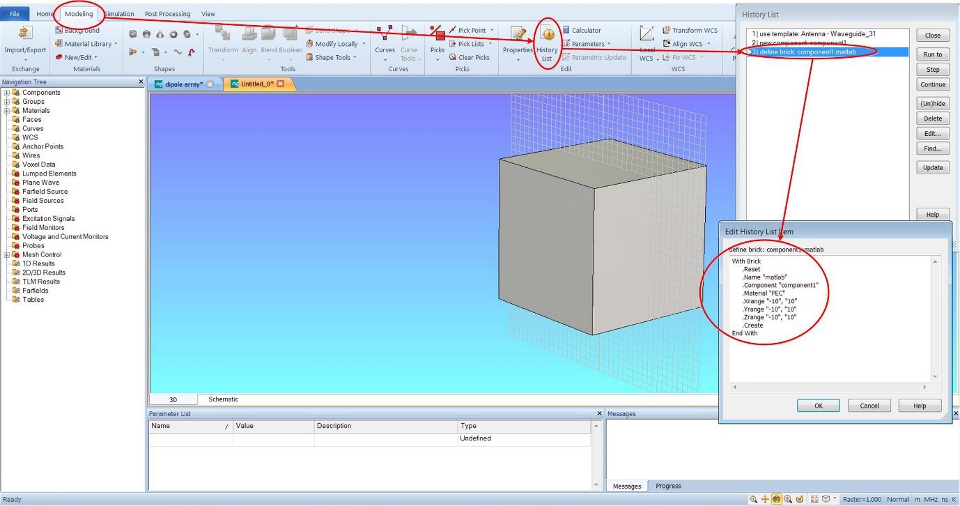
Figure 2 - History List invocation window

Open the Define brick item and turn to its contents and code in Matlab, which allows repeating this sequence of actions.


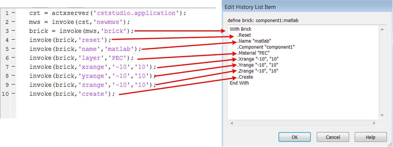
Figure 3 - Define brick window and Matlab code

Figure 3 shows that the code in Matlab is almost a copy of the item from the History List . Thus, it is possible to understand which terminal object should be accessed after selecting the project tab (after the second line of Matlab code) by creating a connection between the CST interface object, in this case Brick , and send commands directly from the History List to this object sequentially .

However, not all commands in the History List have this syntax. For example, the frequency range for calculation is set using the following line:


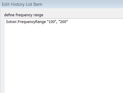
Figure 4 - Setting the frequency range in the History List

Here again, obviously, there is the name of the object to which the commands should be sent - Solver . Then the command to change the frequency range from Matlab will look like this:

solver = invoke(mws,'Solver');
invoke(solver,'FrequencyRange','150','225');

We formulate an algorithm for searching for object names and command format for managing CST Studio from Matlab:

1. It is necessary to perform all the actions that you want to automate in Matlab, from the graphical interface of CST Studio;
2. Open the text of the required operation in the Modeling \ History List (" define brick ", " define frequency range ", etc.);
3. Using the commands below, contact CST Studio from Matlab and open the required file:
   
   

   сst = actxserver('CSTStudio.Application')
   mws = invoke(cst , 'NewMWS') 
   invoke(mws, 'OpenFile', '<Путь к файлу>')

   
   
4. Initialize the connection with the CST Studio object, the parameters of which must be changed, by the header from the History List using the command:
   
   

   <переменная> = invoke(mws, '<Имя объекта>')

5. Enter the commands described in the History List for the object line by line:
   
   

   invoke(<переменная>, '<команда>', '<значение1>', '<значение2>')

This algorithm of actions by trial and error leads to the solution of the problem of managing CST Studio using Matlab code.

Conclusion of analysis results

After the above, you can already send the reader to understand further yourself, but at the very beginning of the article the task was set as inputting the frequency range parameters from Matlab to CST and importing the simulation results as S-transmission parameters back to Matlab. In addition, exporting results to the History List is not displayed.

Using the graphical interface, this is done as follows:

1. After the calculation, select the file in the “tree” of folders to display it;
2. 2 Export it to an ASCII file through the Post Processing \ Import / Export \ Plot Data (ASCII) tab .

Now with Matlab commands you need to do the same.

The team has already been mentioned

invoke(mws,'SelectTreeItem','1D Results/S-Parameters/S1,1')

allowing you to select the desired file in the "tree" of the working field. To display the results in ASCII, we use the built-in CST function “ ASCIIExport ”.
From the help to the CST, in order to perform this function, the following commands must be sent to the CST:

export = invoke(mws,'ASCIIExport')

- initialization of the export function with the variable export;

invoke(export,'reset')

- reset all internal parameters to default values;

invoke(export,'FileName','C:/Result.txt')

- setting the save path and file name;

invoke(export,'Mode','FixedNumber')

- selection of the method of saving points. FixedNumber - displays a strictly specified number of points; FixedWidth - displays points through a given step;

invoke(export,'step','1001')

- number of points for output / step width;

invoke(export,'execute')

- withdrawal command.

This set of commands will allow you to display the reflection coefficient S ₁₁ in the amount of 1001 points in a file located on drive C with the name Results.txt
Thus, the task originally set was completely solved.

Used Books

[1] Potemkin, Valery Georgievich Introduction to MATLAB / V.G. Potemkin. - Moscow: Dialog-MEPhI, 2000 .-- 247 p.: Tab. - ISBN 5-86404-140-8
[2] Reference materials supplied with the CST Studio Suite