RandLib. C ++ 17 probability distribution library
- Tutorial
The RandLib library allows you to work with more than 50 well-known distributions, continuous, discrete, two-dimensional, cyclic, and even one singular. If you need some kind of distribution, then enter its name and add the suffix Rand. Interested in?
Random Generators
If we want to generate a million random variables from a normal distribution using the standard C ++ template library, we will write something like
std::random_device rd;
std::mt19937 gen(rd());
std::normal_distribution<> X(0, 1);
std::vector data(1e6);
for (double &var : data)
   var = X(gen);
Six not very intuitive lines. RandLib allows you to halve their number.
NormalRand X(0, 1);
std::vector data(1e6);
X.Sample(data);
If you need only one random standard normally distributed quantity, then this can be done in one line
double var = NormalRand::StandardVariate();
As you can see, RandLib saves the user from two things: choosing a base generator (a function that returns an integer from 0 to a certain RAND_MAX) and choosing a starting position for a random sequence (srand () function). This is done in the name of convenience, since many users most likely do not need this choice. In the vast majority of cases, random values are generated not directly through the base generator, but through a random value U distributed evenly from 0 to 1, which already depends on this base generator. In order to change the way U is generated, you need to use the following directives:
#define UNIDBLRAND // генератор дает большее разрешение за счет комбинации двух случайных чисел
#define JLKISS64RAND // генератор дает большее разрешение за счет генерации 64-битных целых чисел
#define UNICLOSEDRAND // U может вернуть 0 или 1
#define UNIHALFCLOSEDRAND // U может вернуть 0, но никогда не вернет 1
By default, U returns neither 0 nor 1.
Generation rate
The following table provides a comparison of the time to generate one random variable in microseconds.
System specifications
Ubuntu 16.04 LTS
Processor: Intel Core i7-4710MQ CPU @ 2.50GHz × 8
OS Type: 64-bit
Processor: Intel Core i7-4710MQ CPU @ 2.50GHz × 8
OS Type: 64-bit
| Distribution | STL | Randlib |
|---|---|---|
| 0.017 μs | 0.006 μs |
| 0.075 μs | 0.018 μs |
| 0.109 μs | 0.016 μs |
| 0.122 μs | 0.024 μs |
| 0.158 μs | 0.101 μs |
| 0.108 μs | 0.019 μs |


More comparisons
| Gamma distribution: | ||
|---|---|---|
| 0.207 μs | 0.09 μs |
| 0.161 μs | 0.016 μs |
| 0.159 μs | 0.032 μs |
| 0.159 μs | 0.03 μs |
| 0.159 μs | 0.082 μs |
| Student distribution: | ||
| 0.248 μs | 0.107 μs |
| 0.262 μs | 0.024 μs |
| 0.33 μs | 0.107 μs |
| 0.236 μs | 0.039 μs |
| 0.233 μs | 0.108 μs |
| Fisher Distribution: | ||
| 0.361 μs | 0.099 μs |
| 0.319 μs | 0.013 μs |
| 0.314 μs | 0.027 μs |
| 0.331 μs | 0.169 μs |
| 0.333 μs | 0.177 μs |
| Binomial distribution: | ||
| 0.655 μs | 0.033 μs |
| 0.444 μs | 0.093 μs |
| 0.873 μs | 0.197 μs |
| Poisson distribution: | ||
| 0.048 μs | 0.015 μs |
| 0.446 μs | 0.105 μs |
| Negative binomial distribution: | ||
| 0.297 μs | 0.019 μs |
| 0.587 μs | 0.257 μs |
| 1.017 μs | 0.108 μs |


As you can see, RandLib is sometimes 1.5 times faster than STL, sometimes 2, sometimes 10, but never slower. Examples of algorithms implemented in RandLib can be viewed here and here .
Distribution Functions, Moments, and Other Properties
In addition to generators, RandLib provides the ability to calculate probability functions for any of these distributions. For example, to find out the probability that a random variable with a Poisson distribution with parameter a takes the value k, you need to call function P.
int a = 5, k = 1;
PoissonRand X(a);
X.P(k); // 0.0336897
It so happened that it is the capital letter P that designates the function that returns the probability of taking any value for a discrete distribution. For continuous distributions, this probability is zero almost everywhere; therefore, instead, we consider the density, which is denoted by the letter f. In order to calculate the distribution function for both continuous and discrete distributions, you need to call the function F:
double x = 0;
NormalRand X(0, 1);
X.f(x); // 0.398942
X.F(x); // 0
Sometimes you need to calculate the function 1-F (x), where F (x) takes very small values. In this case, in order not to lose accuracy, the function S (x) should be called.
If you need to calculate the probabilities for a whole set of values, then you need to call the functions:
//x и y - std::vector
X.CumulativeDistributionFunction(x, y); // y = F(x)
X.SurvivalFunction(x, y); // y = S(x)
X.ProbabilityDensityFunction(x, y) // y = f(x) - для непрерывных
X.ProbabilityMassFunction(x, y) // y = P(x) - для дискретных
A quantile is a function of p that returns x such that p = F (x). Corresponding implementations are also in each finite RandLib class corresponding to a one-dimensional distribution:
X.Quantile(p); // возвращает x = F^(-1)(p)
X.Quantile1m(p); // возвращает x = S^(-1)(p)
X.QuantileFunction(x, y) // y = F^(-1)(x)
X.QuantileFunction1m(x, y) // y = S^(-1)(x)
Sometimes instead of the functions f (x) or P (k) it is necessary to get the corresponding logarithms. In this case, it is best to use the following functions:
X.logf(k); // возвращает x = log(f(k))
X.logP(k); // возвращает x = log(P(k))
X.LogProbabilityDensityFunction(x, y) // y = logf(x) - для непрерывных
X.LogProbabilityMassFunction(x, y) // y = logP(x) - для дискретных
RandLib also provides the ability to calculate the characteristic function:
![$ \ phi_X (t) = \ mathbb {E} [e ^ {itX}] $](https://habrastorage.org/getpro/habr/formulas/698/174/6cc/6981746cce77afe38de30d073af8544c.svg)
X.CF(t); // возвращает комплексное значение \phi(t)
X.CharacteristicFunction(x, y) // y = \phi(x)
In addition, you can easily get the first four points or expectation, variance, asymmetry coefficients and kurtosis. In addition, the median (F ^ (- 1) (0.5)) and mode (the point where f or P takes on the greatest value).
LogNormalRand X(1, 1);
std::cout << " Mean = " << X.Mean()
          << " and Variance = " << X.Variance()
          << "\n Median = " << X.Median()
          << " and Mode = " << X.Mode()
          << "\n Skewness = " << X.Skewness()
          << " and Excess kurtosis = " << X.ExcessKurtosis();
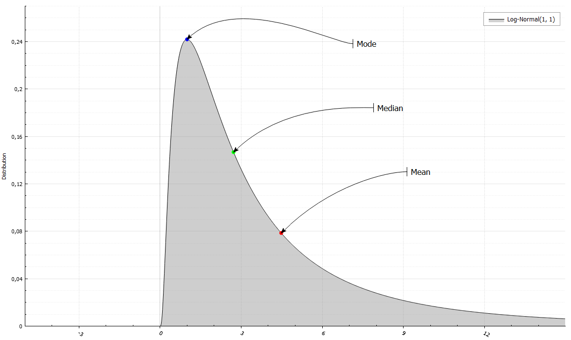
Mean = 4.48169 and Variance = 34.5126
Median = 2.71828 and Mode = 1
Skewness = 6.18488 and Excess Kurtosis = 110.936
Parameter Estimates and Statistical Tests
From probability theory to statistics. For some (not yet for all) classes, there is a Fit function that sets the parameters corresponding to some estimate. Consider the example of a normal distribution:
using std::cout;
NormalRand X(0, 1);
std::vector data(10);
X.Sample(data);
cout << "True distribution: " << X.Name() << "\n";
cout << "Sample: ";
for (double var : data)
    cout << var << "  ";
We generated 10 elements from the standard normal distribution. The output should get something like:
True distribution: Normal(0, 1)
Sample: -0.328154  0.709122  -0.607214  1.11472  -1.23726  -0.123584  0.59374  -1.20573  -0.397376  -1.63173
The Fit function in this case will set the parameters corresponding to the maximum likelihood estimate:
X.Fit(data);
cout << "Maximum-likelihood estimator: " << X.Name(); // Normal(-0.3113, 0.7425)
As is known, the maximum likelihood for the variance of the normal distribution gives a biased estimate. Therefore, the Fit function has an additional unbiased parameter (false by default), which can be used to adjust the bias / non-bias of the estimate.
X.Fit(data, true);
cout << "UMVU estimator: " << X.Name(); // Normal(-0.3113, 0.825)
For fans of Bayesian ideology, there is also a Bayesian assessment. The RandLib structure makes it very convenient to operate with a priori and a posteriori distributions:
NormalInverseGammaRand prior(0, 1, 1, 1);
NormalInverseGammaRand posterior = X.FitBayes(data, prior);
cout << "Bayesian estimator: " << X.Name(); // Normal(-0.2830, 0.9513)
cout << "(Posterior distribution: " << posterior.Name() << ")"; //  Normal-Inverse-Gamma(-0.2830, 11, 6, 4.756)
Tests
How do you know that generators, like distribution functions, return the correct values? Answer: compare one with another. For continuous distributions, a function is implemented that conducts the Kolmogorov-Smirnov test for the membership of this sample in the corresponding distribution. The KolmogorovSmirnovTest function accepts ordinal statistics and the \ alpha level as input, and returns true if the selection matches the distribution. Discrete distributions correspond to the PearsonChiSquaredTest function.
Conclusion
This article is specifically written for the part of the habrasociety, interested in this and able to appreciate. Understand, poking around, use your health. The main advantages:
- Free
- Open source
- Work speed
- Ease of use (my subjective opinion)
- No dependencies (yes, nothing is needed)
Link to the release .