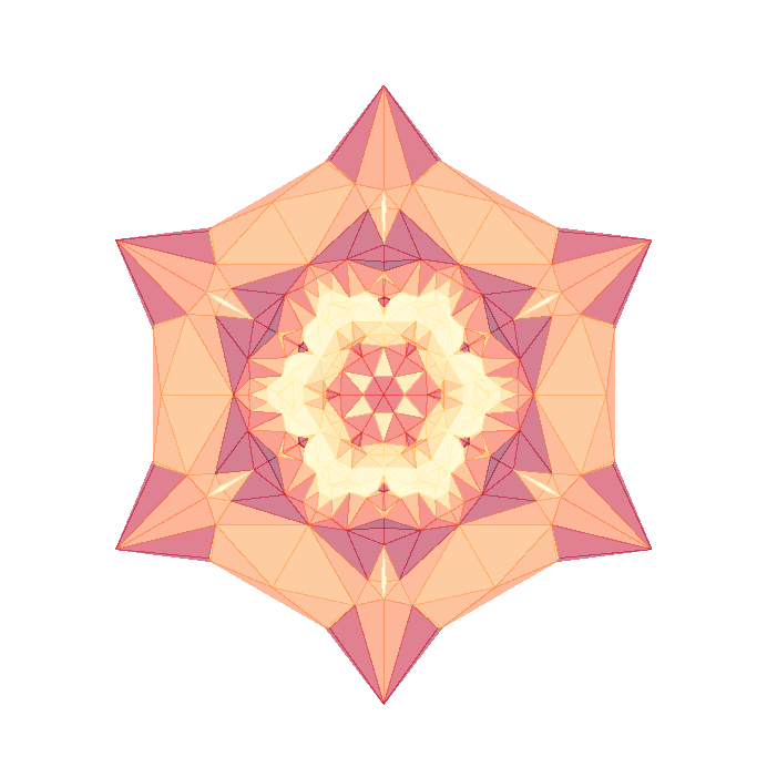
Saltan Spectroscope: Laplacians for a fan
Christmas days - time to put aside your usual affairs and remember fun - kaleidoscopes, mosaics, snowflakes ... Who will draw the most beautiful star?
Symmetry pleases the eye. Mathematics helps to create beauty, the Python language and its libraries - mathematical numpy and graphic matplotlib .
KDPV is obtained by visualizing the values of the eigenvectors of a certain symmetric matrix.
The basis is the spectra of regular lattices. Some of their properties have already been considered previously . Here the formulas work for aesthetics.
So, let's say there is a certain basic set of points located on a plane. There are few requirements - the configuration should be centrally symmetrical. For example, a hexagonal grid would be a good choice:
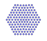
Already beautiful, only somewhat monotonous.
Mugs are dots. Each is characterized by two coordinates. For a given set of points, you can calculate their own coordinates based on the matrix of squares of the distances between the points. This is described in the above article. To calculate the spectrum, it is necessary to transform the matrix of squares of distances into the Laplacian (which in this case is the correlation matrix) and calculate the spectrum of this Laplacian, that is, find its eigenvalues and the corresponding vectors.
If we calculate the spectrum for a set of points located on the plane, then there will be only two components in the spectrum - one corresponds to the x coordinate, and the other corresponds to y.
But it is necessary to make the spectrum “ring”, but at the same time retain the symmetry. This is easy to achieve. It is enough to change (or outrage) the function of the distance between points. For example, we can assume that the distance between the points is not equal to the square of the distance, but to its cube, or the reciprocal of the distance — you can use any function that depends on the distance.
For such a "matrix of distances" the spectrum can no longer be two-dimensional. The algorithm for decomposing the distance matrix into a spectrum must somehow select for each point such a set of coordinates to satisfy a non-standard distance. Such a spectrum begins to ring, - the number of its components in the general case is equal to the total number of points (however, zero can be excluded).
If the set of points is symmetric, then part of the components will be degenerate. This means that the same value of the eigenvalue will correspond to different eigenvectors. In our case, the initial configuration of the points is two-dimensional, respectively, and the degree of degeneracy will be a multiple of two (probably, there is some kind of theorem for this statement). And this means that such doubly degenerate levels - projections - can be drawn on a plane. In the simplest version, also with dots.
Suppose that the distance function has the following form:
f (R2) = w * Rd + 1 / Rd , where w = dist / n ^ 2, Rd = R2 ^ degree .
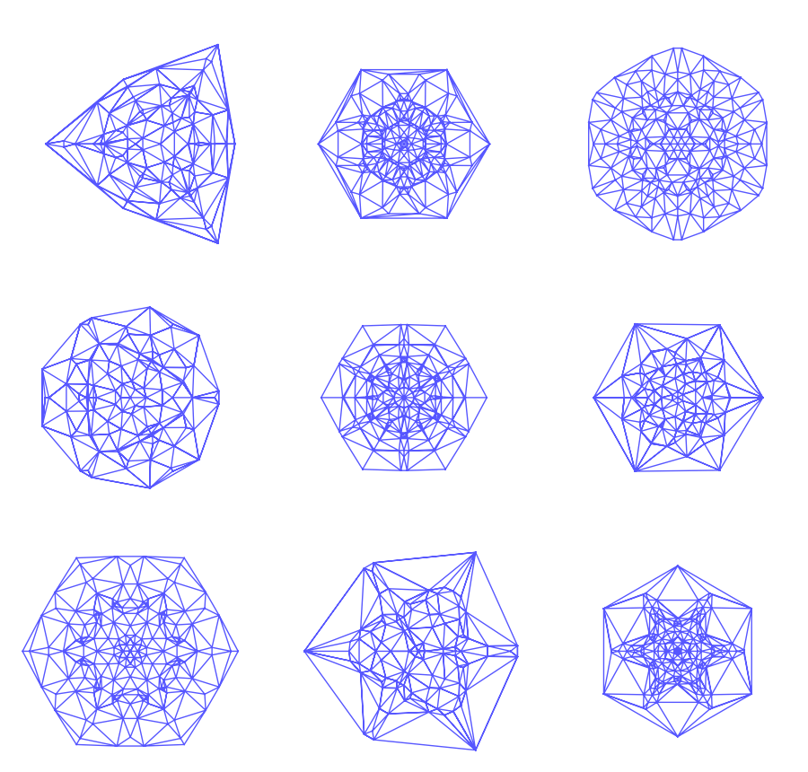
Here dist and degree- two variable perturbation parameters. Then the first 9 degenerate levels for the above basic configuration (hexagonal lattice of size 7) with the perturbation parameters dist = -2 , degree = 1 are:
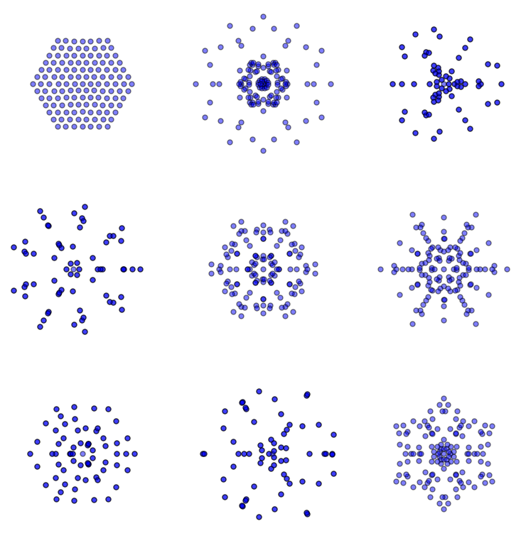
In the upper left corner - the initial configuration. The parameter values are selected so that it is almost not distorted.
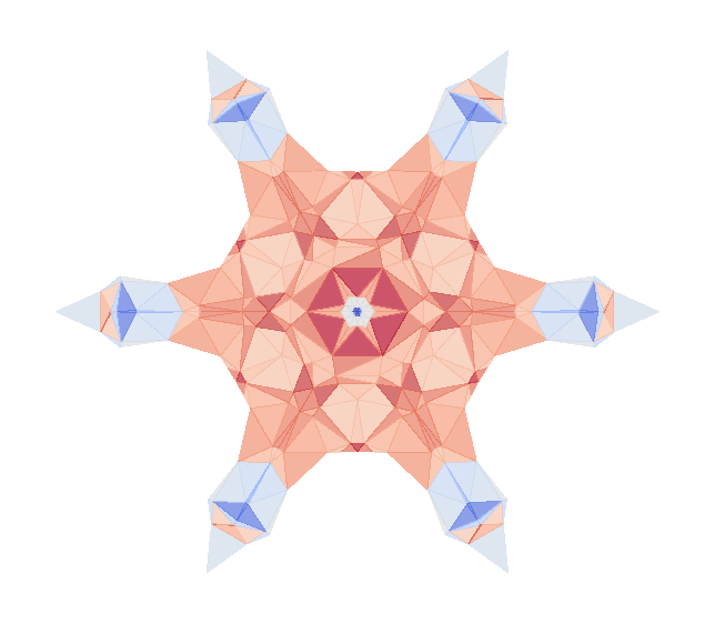
All patterns are guaranteed to be different, this follows from the properties of eigenvectors (although sometimes they are not distinguishable by eye). Some seem more unusual than others. Here, for example, one of the bizarre configurations:

You can take a square lattice as an initial set. Then the symmetry will be square:
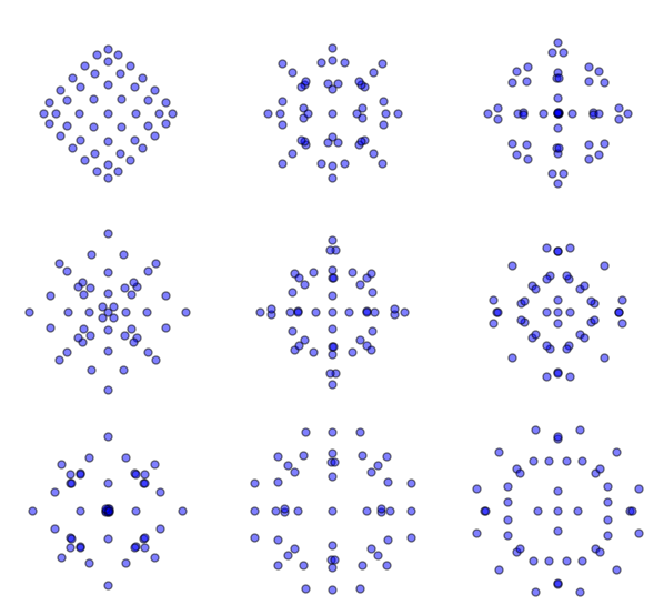
Since the symmetry is reduced, the number of non-degenerate spectra here is twice as many as degenerate.
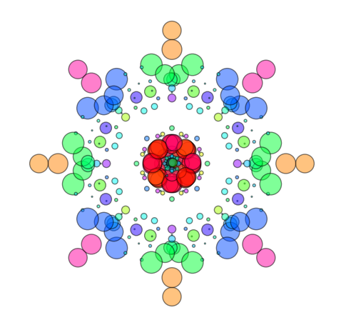
If you give the dots color and size, then the snowflakes (patterns) will become more fun and diverse. The trick is that the color and size of the points can also be formed on the basis of the eigenvectors of this set.
The color generation algorithm is simple. We use a certain color map (from the available sets in matplotlib ), which converts the value of the point to color, and we take the value of the point from some non-degenerate eigenvector. The same goes for point size. Then you can get something like this fun lace:
If you vary only the color, you can play a children's mosaic:
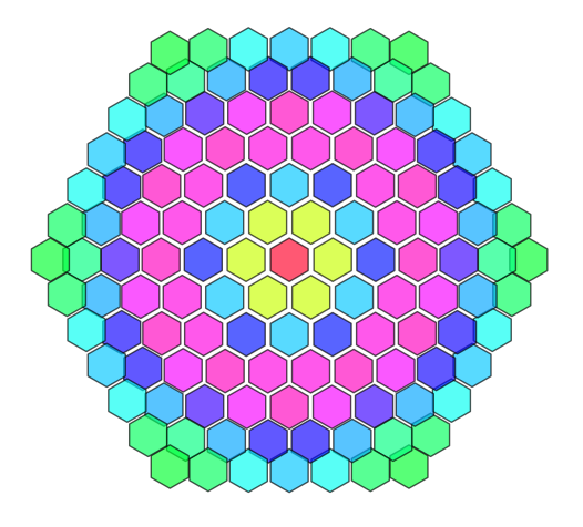
This is the mathematics that painted the basic configuration of the dots in different colors.
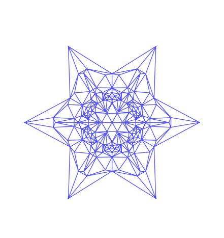
If close points are connected by lines, then we get something like a web. Scientifically, such an operation is called triangulation . The advantage of the matplotlib package is that there such an operation is available “out of the box”. The cobwebs are beautiful:
You can remove part of the triangles based on the masks :
Triangulation becomes colored if triangles are filled with different colors:
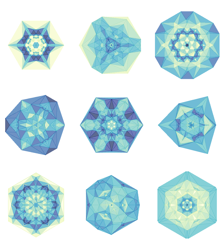
Choosing a color map and a color vector greatly affects the perception of the same configuration:

Using masks sharpen the contours of the patterns: The
number of combinations and variations is almost infinite, the play of patterns is very bizarre.
Perhaps the most exquisite are the patterns obtained by drawing contours based on triangulation. These patterns are obtained using the tricontour () method of the matplotlib library. Even the most ordinary-looking and boring sets of points acquire completely unexpected variations.

Symmetry can be any, for example, of the 5th order:
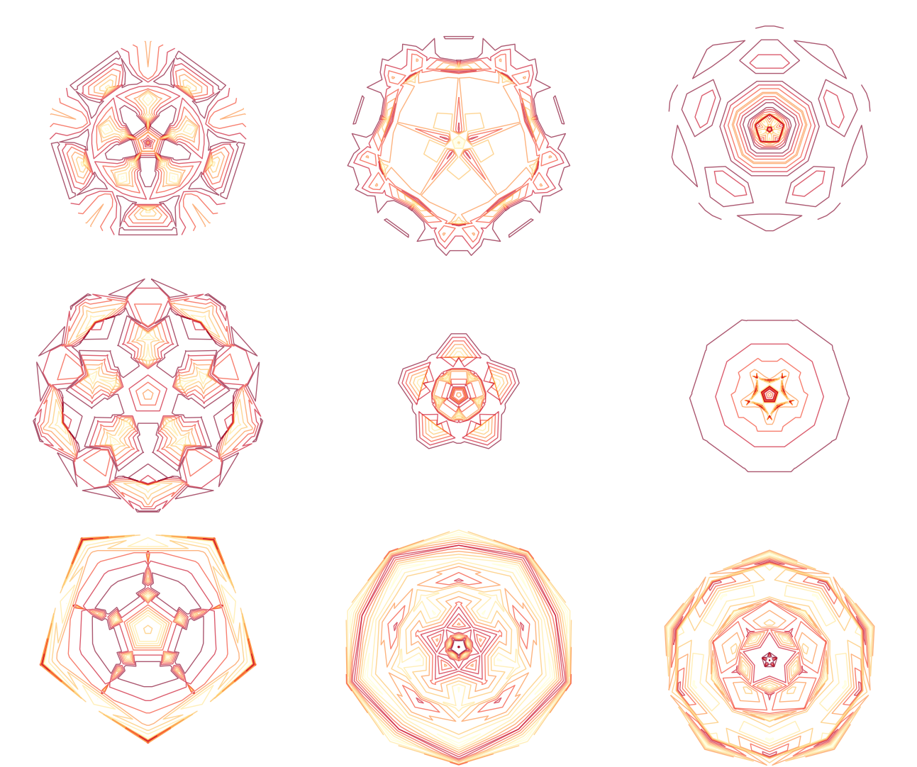
some kind of magic.
All of these patterns were created using the program " Spectroscope " written in Python. The program code is not perfect, but accessible .
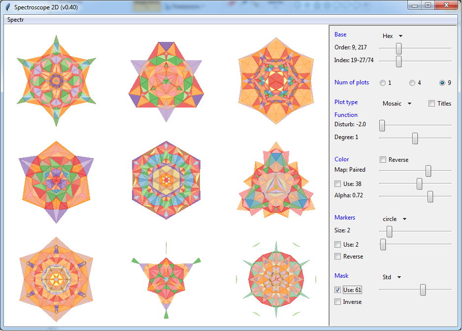
With its help, anyone can create patterns by varying parameters through a simple interface.
At the top of the control panel, you can select one of the basic sets of point distributions ( Base ). The base distribution always has an index of one if the perturbation parameters are -2 ( Disturb ) and 1 ( Degree ), respectively , so you can always look at it.
The most powerful are the basic sets of Hex (hex) and Square(square), since they have the most points. Therefore, they give more diverse patterns. But the sets x-border (polygon borders) and especially Circle (circle), on the contrary, are emasculated and more interesting for research purposes.
For a basic set, you can specify its size ( Order ) using the slider (slider). The next field ( Index ) sets the numbers of the displayed spectra (levels) from those available for this set. In this version, you can display 1, 4 or 9 patterns at the same time.
An important parameter is the type of pattern ( Plot type ). It is he who sets the way (mode) of displaying our own vectors. Available are listed above ( Points, Web, Mosaic, Contour ).
The " Titles " checkbox displays over each spectrum its numerical parameters, serial number in the overall composition of the levels and the eigenvalue of the given level. This is for those who are interested in more than just graphics.
Below are two sliders for the variation parameters. When they change, the spectra come to life. Recall that the right mouse button on the slider - shifts it to the current position, the left - increments.
The following are the parameters that affect the appearance of the spectra - color, markers and mask. Not all display modes are involved. Markers, for example, are relevant only for the "point" mode, and masks - on the contrary - for all but the point mode.
Perhaps the most important is the color (Color). To set it, you must specify a color map (Map). But they play with color using the vector (slider with the Use flag). The color vector (and marker size too) is selected, as already noted, from non-degenerate levels.
Standard functions are available in the program menu for saving spectra to files and exporting as images.
There are many areas where you can develop a spectroscope. In addition to obvious improvements to the interface, the development of features (animation, for example, or web access), you need to try to build three-dimensional patterns. They can not only be watched, but also sculpted).
During games with spectra, several interesting questions of varying degrees of importance arise.
Maybe this is not the most important question, but perhaps the simplest. Obviously, the fraction of degenerate spectra depends on the basic distribution of points. There are explicit formulas for the main lattices (hexagonal and square).
For a hexagonal lattice, the number of “snowflakes” Ns is related to the total number of points (nodes) N as:
Ns = (N-1) / 3
In turn, the number of points quadratically depends on the size of the lattice a :
N (a) = 3a (a-1 ) + 1 . Hence Ns (a) = a (a-1).
In a square lattice, the number of degenerate spectra is related to the number of points in a similar way:
Ns = N / 4 = a ^ 2/4
How to obtain such formulas for arbitrary configurations is not very clear. It is possible that a general algorithm does not exist.
Perhaps the most interesting question. The main way to identify the levels of the spectrum is the value of the eigenvalue. If you sort these numbers in ascending order, you can assign an index to each level (eigenvalue value). This index seems to identify the spectrum.
This is actually not a very reliable way. When the perturbation parameters are varied, the spectra come to life - the patterns begin to breathe (for example, you can see how the “base” distribution “flattens” when the Disturb parameter changes), and their eigenvalues also change. In this case, situations arise when the eigenvalues of different levels approach each other and pass on. That is, the spectra change places. Moreover, by the nature of the spectrum pattern, one can see where is which spectrum. This "character" and must somehow be hashed into the identifier of the spectrum.
The phenomenon of rapid changes in patterns occurs in a narrow band of the perturbation parameter. Something like a phase transition. It is possible that this is a known phenomenon. During the phase transition, both the form of the spectra and their relative location change. In the program, the form of the perturbed function is chosen so that when the Disturb perturbation parameter changes, the function changes sign. You can see that the basic distribution when changing the parameter from minimum to maximum goes from the first index to the last. This transition seems to be carried out by moving the base pattern in the indexes from the smallest to the largest. After some time, the changed base pattern appears at the last index. Which then evolves to the original base configuration.
However, in large configurations, it seems that no one is moving anywhere (well, or it is impossible to track). Just at a certain moment, the rudiment of a new basic configuration arises in the right place (at the maximum index). In short, anyone interested - take a look).
If there was any parameter for identifying the proper levels, it would be possible to more accurately track the movement (or death and birth?) Of the spectra. And always show the specified spectra in the picture, regardless of the values of their eigenvalues.
also not yet very successful. Patterns periodically rotate left / right. It is not clear how the easiest way to orient them is always in one direction.
When the basic configuration is a simple circle (points at the vertices of regular polygons), the phenomenon of integer divisors arises. In this configuration, all points are equal. Accordingly, all degenerate levels (and there are no others here) are also the coordinates of the vertices of the polygons (lie on a circle). But at the same time, the spectra of simple polygons (the number of vertices are a prime number) differ from composite ones. In the spectra of primes, all levels are also simple polygons with the same number of vertices. And in the spectra of composite levels consist of divisors of the vertices of the base polygon.
For example, the spectrum of a 30-gon consists of 14 degenerate levels (projections). Of these, four 30-gons, four 15-gons, two 10-gons, one 6-gon, two 5-gons and one 3-gon. Why such a distribution of levels by divisors is not clear (but they didn’t penetrate much). Perhaps this has already been explained somewhere in group theory.
That's all for now. Good luck with your creative search and Merry Christmas!
Symmetry pleases the eye. Mathematics helps to create beauty, the Python language and its libraries - mathematical numpy and graphic matplotlib .
Spectra of impossible gratings
KDPV is obtained by visualizing the values of the eigenvectors of a certain symmetric matrix.
The basis is the spectra of regular lattices. Some of their properties have already been considered previously . Here the formulas work for aesthetics.
So, let's say there is a certain basic set of points located on a plane. There are few requirements - the configuration should be centrally symmetrical. For example, a hexagonal grid would be a good choice:
Already beautiful, only somewhat monotonous.
Mugs are dots. Each is characterized by two coordinates. For a given set of points, you can calculate their own coordinates based on the matrix of squares of the distances between the points. This is described in the above article. To calculate the spectrum, it is necessary to transform the matrix of squares of distances into the Laplacian (which in this case is the correlation matrix) and calculate the spectrum of this Laplacian, that is, find its eigenvalues and the corresponding vectors.
If we calculate the spectrum for a set of points located on the plane, then there will be only two components in the spectrum - one corresponds to the x coordinate, and the other corresponds to y.
But it is necessary to make the spectrum “ring”, but at the same time retain the symmetry. This is easy to achieve. It is enough to change (or outrage) the function of the distance between points. For example, we can assume that the distance between the points is not equal to the square of the distance, but to its cube, or the reciprocal of the distance — you can use any function that depends on the distance.
For such a "matrix of distances" the spectrum can no longer be two-dimensional. The algorithm for decomposing the distance matrix into a spectrum must somehow select for each point such a set of coordinates to satisfy a non-standard distance. Such a spectrum begins to ring, - the number of its components in the general case is equal to the total number of points (however, zero can be excluded).
If the set of points is symmetric, then part of the components will be degenerate. This means that the same value of the eigenvalue will correspond to different eigenvectors. In our case, the initial configuration of the points is two-dimensional, respectively, and the degree of degeneracy will be a multiple of two (probably, there is some kind of theorem for this statement). And this means that such doubly degenerate levels - projections - can be drawn on a plane. In the simplest version, also with dots.
Suppose that the distance function has the following form:
f (R2) = w * Rd + 1 / Rd , where w = dist / n ^ 2, Rd = R2 ^ degree .
Here dist and degree- two variable perturbation parameters. Then the first 9 degenerate levels for the above basic configuration (hexagonal lattice of size 7) with the perturbation parameters dist = -2 , degree = 1 are:
In the upper left corner - the initial configuration. The parameter values are selected so that it is almost not distorted.
All patterns are guaranteed to be different, this follows from the properties of eigenvectors (although sometimes they are not distinguishable by eye). Some seem more unusual than others. Here, for example, one of the bizarre configurations:
You can take a square lattice as an initial set. Then the symmetry will be square:
Since the symmetry is reduced, the number of non-degenerate spectra here is twice as many as degenerate.
Add color and size.
If you give the dots color and size, then the snowflakes (patterns) will become more fun and diverse. The trick is that the color and size of the points can also be formed on the basis of the eigenvectors of this set.
The color generation algorithm is simple. We use a certain color map (from the available sets in matplotlib ), which converts the value of the point to color, and we take the value of the point from some non-degenerate eigenvector. The same goes for point size. Then you can get something like this fun lace:
If you vary only the color, you can play a children's mosaic:
This is the mathematics that painted the basic configuration of the dots in different colors.
Cobwebs
If close points are connected by lines, then we get something like a web. Scientifically, such an operation is called triangulation . The advantage of the matplotlib package is that there such an operation is available “out of the box”. The cobwebs are beautiful:
You can remove part of the triangles based on the masks :
Mosaics
Triangulation becomes colored if triangles are filled with different colors:
Choosing a color map and a color vector greatly affects the perception of the same configuration:
Using masks sharpen the contours of the patterns: The
number of combinations and variations is almost infinite, the play of patterns is very bizarre.
Outlines
Perhaps the most exquisite are the patterns obtained by drawing contours based on triangulation. These patterns are obtained using the tricontour () method of the matplotlib library. Even the most ordinary-looking and boring sets of points acquire completely unexpected variations.
Symmetry can be any, for example, of the 5th order:
some kind of magic.
Spectroscope
All of these patterns were created using the program " Spectroscope " written in Python. The program code is not perfect, but accessible .
With its help, anyone can create patterns by varying parameters through a simple interface.
At the top of the control panel, you can select one of the basic sets of point distributions ( Base ). The base distribution always has an index of one if the perturbation parameters are -2 ( Disturb ) and 1 ( Degree ), respectively , so you can always look at it.
The most powerful are the basic sets of Hex (hex) and Square(square), since they have the most points. Therefore, they give more diverse patterns. But the sets x-border (polygon borders) and especially Circle (circle), on the contrary, are emasculated and more interesting for research purposes.
For a basic set, you can specify its size ( Order ) using the slider (slider). The next field ( Index ) sets the numbers of the displayed spectra (levels) from those available for this set. In this version, you can display 1, 4 or 9 patterns at the same time.
An important parameter is the type of pattern ( Plot type ). It is he who sets the way (mode) of displaying our own vectors. Available are listed above ( Points, Web, Mosaic, Contour ).
The " Titles " checkbox displays over each spectrum its numerical parameters, serial number in the overall composition of the levels and the eigenvalue of the given level. This is for those who are interested in more than just graphics.
Below are two sliders for the variation parameters. When they change, the spectra come to life. Recall that the right mouse button on the slider - shifts it to the current position, the left - increments.
The following are the parameters that affect the appearance of the spectra - color, markers and mask. Not all display modes are involved. Markers, for example, are relevant only for the "point" mode, and masks - on the contrary - for all but the point mode.
Perhaps the most important is the color (Color). To set it, you must specify a color map (Map). But they play with color using the vector (slider with the Use flag). The color vector (and marker size too) is selected, as already noted, from non-degenerate levels.
Standard functions are available in the program menu for saving spectra to files and exporting as images.
There are many areas where you can develop a spectroscope. In addition to obvious improvements to the interface, the development of features (animation, for example, or web access), you need to try to build three-dimensional patterns. They can not only be watched, but also sculpted).
Mathematical aspects
During games with spectra, several interesting questions of varying degrees of importance arise.
Calculation of the number of degenerate spectra
Maybe this is not the most important question, but perhaps the simplest. Obviously, the fraction of degenerate spectra depends on the basic distribution of points. There are explicit formulas for the main lattices (hexagonal and square).
For a hexagonal lattice, the number of “snowflakes” Ns is related to the total number of points (nodes) N as:
Ns = (N-1) / 3
In turn, the number of points quadratically depends on the size of the lattice a :
N (a) = 3a (a-1 ) + 1 . Hence Ns (a) = a (a-1).
In a square lattice, the number of degenerate spectra is related to the number of points in a similar way:
Ns = N / 4 = a ^ 2/4
How to obtain such formulas for arbitrary configurations is not very clear. It is possible that a general algorithm does not exist.
Spectrum Level Identification
Perhaps the most interesting question. The main way to identify the levels of the spectrum is the value of the eigenvalue. If you sort these numbers in ascending order, you can assign an index to each level (eigenvalue value). This index seems to identify the spectrum.
This is actually not a very reliable way. When the perturbation parameters are varied, the spectra come to life - the patterns begin to breathe (for example, you can see how the “base” distribution “flattens” when the Disturb parameter changes), and their eigenvalues also change. In this case, situations arise when the eigenvalues of different levels approach each other and pass on. That is, the spectra change places. Moreover, by the nature of the spectrum pattern, one can see where is which spectrum. This "character" and must somehow be hashed into the identifier of the spectrum.
Phase transitions
The phenomenon of rapid changes in patterns occurs in a narrow band of the perturbation parameter. Something like a phase transition. It is possible that this is a known phenomenon. During the phase transition, both the form of the spectra and their relative location change. In the program, the form of the perturbed function is chosen so that when the Disturb perturbation parameter changes, the function changes sign. You can see that the basic distribution when changing the parameter from minimum to maximum goes from the first index to the last. This transition seems to be carried out by moving the base pattern in the indexes from the smallest to the largest. After some time, the changed base pattern appears at the last index. Which then evolves to the original base configuration.
However, in large configurations, it seems that no one is moving anywhere (well, or it is impossible to track). Just at a certain moment, the rudiment of a new basic configuration arises in the right place (at the maximum index). In short, anyone interested - take a look).
If there was any parameter for identifying the proper levels, it would be possible to more accurately track the movement (or death and birth?) Of the spectra. And always show the specified spectra in the picture, regardless of the values of their eigenvalues.
Image stabilization
also not yet very successful. Patterns periodically rotate left / right. It is not clear how the easiest way to orient them is always in one direction.
Dividers
When the basic configuration is a simple circle (points at the vertices of regular polygons), the phenomenon of integer divisors arises. In this configuration, all points are equal. Accordingly, all degenerate levels (and there are no others here) are also the coordinates of the vertices of the polygons (lie on a circle). But at the same time, the spectra of simple polygons (the number of vertices are a prime number) differ from composite ones. In the spectra of primes, all levels are also simple polygons with the same number of vertices. And in the spectra of composite levels consist of divisors of the vertices of the base polygon.
For example, the spectrum of a 30-gon consists of 14 degenerate levels (projections). Of these, four 30-gons, four 15-gons, two 10-gons, one 6-gon, two 5-gons and one 3-gon. Why such a distribution of levels by divisors is not clear (but they didn’t penetrate much). Perhaps this has already been explained somewhere in group theory.
That's all for now. Good luck with your creative search and Merry Christmas!