How to solve simple optimization problems in python using cvxpy
Good day to all! With a simple search, I could not find the mention of the cvxpy module and therefore decided to write training material on it - just code examples, according to which it will be easier for a beginner to use this module for his tasks. cvxpy is designed to solve optimization problems - finding minima / maxima of functions with certain restrictions. If you are interested in this topic - I ask for a cat.

Here x is an independent variable (in the general case, a vector), f (x) is the
objective function that needs to be optimized. Restrictions on the domain of definition of f (x) can be specified using equalities and inequalities.
Let's look at the following linear programming problem :
If you look at the area defined by the inequality with the module, you can see that this area can easily be defined using linear inequalities:
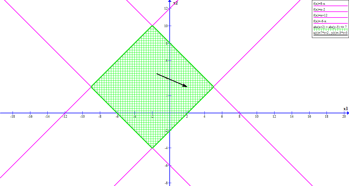
In our case, the restrictions will be as follows:

The module installation is described in detail on the module website . Let's write a simple code that will allow us to solve our test optimization problem:
Our current solution is not integral and goes beyond the limitations, but it can be seen that it lies next to the optimal solution (-9, 3) . In cvxpy, you can use different solvers to solve the problem, choosing the best one. Let's try GLPK :
The list of available solvers is returned by the function
It is possible to solve not only linear programming problems. Let's look at the initial statement of the problem:
You can also look for a solution for the least squares method :
Of course, some tasks may have a trivial solution:
And some may not have a solution at all:
That's all. You can find out more on the module website .
General statement of the problem
Here x is an independent variable (in the general case, a vector), f (x) is the
objective function that needs to be optimized. Restrictions on the domain of definition of f (x) can be specified using equalities and inequalities.
Task example
Let's look at the following linear programming problem :
If you look at the area defined by the inequality with the module, you can see that this area can easily be defined using linear inequalities:
In our case, the restrictions will be as follows:
Solving a problem using cvxpy
The module installation is described in detail on the module website . Let's write a simple code that will allow us to solve our test optimization problem:
import numpy as np
import cvxpy as cvx
# наши независимые переменные
x = cvx.Variable(2)
A = np.array([[1, 1],
              [1, -1],
              [-1, 1],
              [-1, -1]])
b = np.array([8, 2, 12, 6])
c = np.array([7, -3])
# ограничения
constraints = [A * x <= b]
# целевая функция и что с ней делать
obj = cvx.Minimize(c * x)
# формулируем задачу и решаем
prob = cvx.Problem(obj, constraints)
prob.solve()
print(prob.status) # optimal
print(prob.value) # -71.999999805
print(x.value) # [[-8.99999997] [ 3.00000002]]
Our current solution is not integral and goes beyond the limitations, but it can be seen that it lies next to the optimal solution (-9, 3) . In cvxpy, you can use different solvers to solve the problem, choosing the best one. Let's try GLPK :
prob.solve(solver = "GLPK")
print(prob.status) # optimal
print(prob.value) # -72.0
print(x.value) # [[-9.] [ 3.]]
The list of available solvers is returned by the function
installed_solvers().Other examples
It is possible to solve not only linear programming problems. Let's look at the initial statement of the problem:
# ограничения
constraints = [cvx.abs(x[0] + 2) + cvx.abs(x[1] - 3) <= 7]
# целевая функция и что с ней делать
obj = cvx.Minimize(c * x)
# формулируем задачу и решаем
prob = cvx.Problem(obj, constraints)
prob.solve(solver = "GLPK")
print(prob.status) # optimal
print(prob.value) # -72.0
print(x.value) # [[-9.] [ 3.]]
You can also look for a solution for the least squares method :
# целевая функция и что с ней делать
obj = cvx.Minimize(cvx.norm(A * x - b)) # по умолчанию используется вторая норма
# формулируем задачу и решаем
prob = cvx.Problem(obj)
prob.solve()
print(prob.status) # optimal
print(prob.value) # 13.9999999869
print(x.value) # [[-2.] [ 3.]]
Of course, some tasks may have a trivial solution:
A = np.array([[1, 1],
              [1, -1],
              [-1, 1]])
b = np.array([8, 2, 12])
c = np.array([7, -3])
# ограничения
constraints = [A * x <= b]
# целевая функция и что с ней делать
obj = cvx.Minimize(c * x)
# формулируем задачу и решаем
prob = cvx.Problem(obj, constraints)
prob.solve()
print(prob.status) # unbounded
print(prob.value) # -inf
print(x.value) # None
And some may not have a solution at all:
A = np.array([[1, 1],
              [1, -1],
              [-1, 1],
              [-1, -1]])
b = np.array([-6, -12, -2, -8])
# ограничения
constraints = [A * x <= b]
# целевая функция и что с ней делать
obj = cvx.Minimize(c * x)
# формулируем задачу и решаем
prob = cvx.Problem(obj, constraints)
prob.solve()
print(prob.status) # infeasible
print(prob.value) # inf
print(x.value) # None
That's all. You can find out more on the module website .