Variational autocoder (autoencoder) is a generative model that learns to map objects into a given hidden space.

Ever wondered how the variational auto-encoder (VAE) model works? Want to know how VAE generates new examples like the data set on which it was trained? After reading this article, you get a theoretical idea of ​​the inner workings of VAE, and you can also implement it yourself. Then, I’ll show you the VAE work code, which is trained on typing handwritten numbers, and we’ll have some fun while generating new numbers!

Generative models

VAE is a generative model — it estimates the probability density (PDF) of the training data. If such a model is trained in natural images, it will assign a high probability value to the lion image, and a low value to the random nonsense image.

The VAE model is also able to take examples from a trained PDF, which is the coolest part, since it will be able to generate new examples similar to the original data set!

I will explain VAE using the MNIST handwritten dialing . The input data for the model are images in the format$$. The model should estimate the likelihood of how the input data looks like a digit.

Image modeling task

The interaction between pixels is a difficult task. If the pixels are independent of each other, then you need to study the PDF of each pixel independently, which is easy. The sample is also simple - we take each pixel separately.

But in digital images there are clear dependencies between pixels. If you see the beginning of the four on the left half, then be very surprised if the right half is the completion of zero. But why?..

Hidden space

You know that on each image there is one digit. Sign in$$does not explicitly contain this information. But it must be somewhere ... This "somewhere" is a hidden space.



You can think of the hidden space as$$where each vector contains $$parts of the information needed to render the image. Suppose the first dimension contains a number represented by a digit. The second dimension can be width. The third is the corner, and so on.

We can imagine the process of drawing a human figure in two steps. First, a person determines, consciously or not, all the attributes of the number that he intends to move. Further, these solutions are transformed into strokes on paper.

VAE is trying to simulate this process: at a given image$$we want to find at least one hidden vector capable of describing it; one vector containing instructions for generating$$. Formulating it according to the formula of total probability , we get$$.

Let's put a reasonable sense into this equation:

• Integral means that candidates must be sought in the entire hidden space.
• For each candidate $$ we ask the question: is it possible to generate $$using instructions $$? Big enough$$? For example, if$$encodes information about the number 7, then image 8 is impossible. However, image 1 is valid because 1 and 7 are similar.
• We found good $$? Fine! But wait a second ... as far as$$ probably? $$big enough? Consider an image of an inverted digit 7. The ideal match would be a hidden vector describing view 7, where the angle size is set to 180 °. However, such$$ unlikely, because usually the numbers do not write at an angle of 180 °.

The goal of VAE training is to maximize $$. We will model$$ using multidimensional Gaussian distribution $$.

$$ modeled using neural network. $$ Is a hyperparameter for multiplying the identity matrix $$.

It should be borne in mind that$$- this is what we will use to generate new images using a trained model. Overlaying a Gaussian distribution is for educational purposes only. If we take the Dirac delta function (i.e. deterministic$$), then we will not be able to train the model using a gradient descent!

Wonders of Hidden Space

The hidden space approach has two big problems:

1. What information does each dimension contain? Some dimensions may refer to abstract elements, such as style. Even if it was easy to interpret all the dimensions, we don’t want to assign labels to the data set. This approach does not scale to other data sets.
2. Hidden space can be confused when there is a correlation between measurements. For example, a very quickly drawn figure can simultaneously lead to the appearance of both angular and thinner strokes. Determining these dependencies is difficult.

Deep learning comes to the rescue

It turns out that each distribution can be generated by applying a fairly complex function on a standard multidimensional Gaussian distribution.

Choose$$as a standard multidimensional Gaussian distribution. Thus, simulated by the neural network$$ can be divided into two phases:

1. The first layers map the Gaussian distribution to the true distribution over the hidden space. We will not be able to interpret the measurement, but it does not matter.
2. Subsequent layers will be displayed from hidden space in $$.

So how do we train this beast?

Formula for $$ insoluble, so we approximate it by the Monte Carlo method:

1. Selection $$ from previous $$
2. Approximation with $$

Fine! So, just try a lot of different$$and start the back propagation party!

Unfortunately, since$$very multidimensional, a lot of samples are required to get a reasonable approximation. I mean, if you try$$what are the chances of getting an image that looks something like $$? This, by the way, explains why$$ must assign a positive probability value to any possible image, otherwise the model will not be able to learn: sampling $$ will lead to an image that is almost certainly different from $$, and if the probability is 0, then the gradients will not be able to spread.

How to solve this problem?

Cut the way!

Most samples $$ from the sample will not add anything to $$ - they are too far beyond its borders. Now, if you knew in advance where to select them ...

You can enter$$. This$$ will be trained to assign high probability values ​​to those $$which are likely to generate $$. Now it is possible to carry out a Monte-Carlo estimation, taking far fewer samples from$$.

Unfortunately, there is a new problem! Instead of maximizing$$ we maximize $$. How are they related to each other?

Variation output

Variational conclusion is the topic of a separate article, so I will not dwell on it here in detail. I can only say that these distributions are related by the following equation:

$$

$$is the Kullback – Leibler distance , which intuitively evaluates the similarity of the two distributions.

After a moment, you will see how to maximize the right side of the equation. At the same time, the left side is also maximized:

• $$ maximized.
• how far $$ from $$- the present prior unknown will be minimized.

The meaning of the right side of the equation is that we have a voltage here:

1. On the one hand, we want to maximize how good $$ must be decoded from $$.
2. On the other hand, we want $$( encoder ) was similar to the previous one$$(multidimensional Gaussian distribution). This can be viewed as a regularization.

Minimization of divergence $$performed easily with the right choice of distributions. We will model$$ as a neural network, the output of which is the parameters of a multi-dimensional Gaussian distribution:

• the average $$
• diagonal covariance matrix $$

Then divergence $$becomes analytically solvable, which is great for us (and for gradients).

Part of the decoder is a bit more complicated. At first glance, I want to say that this task is unsolvable by the Monte Carlo method. But sampling$$ of $$ will not allow gradients to propagate through $$because sampling is not a differentiated operation. This is a problem, since then the weights of the layers that produce$$ and $$.

The trick of the new parameterization

We can replace $$ deterministic parametrized transformation of non-parametric random variable:

1. A sample of the standard (without parameters) Gaussian distribution.
2. Multiply the sample by the square root $$.
3. Adding to the result $$.

As a result, we obtain a distribution equal to $$. Now the sampling operation comes from the standard Gaussian distribution. Therefore, gradients can propagate through$$ and $$, since now these are deterministic paths.

Result? The model will be able to learn how to adjust the parameters.$$: she will concentrate around good $$that are capable of producing $$.

Putting it all together

A VAE model can be hard to understand. We looked at a lot of material here that is hard to digest.

Let me summarize all the steps for implementing VAE.



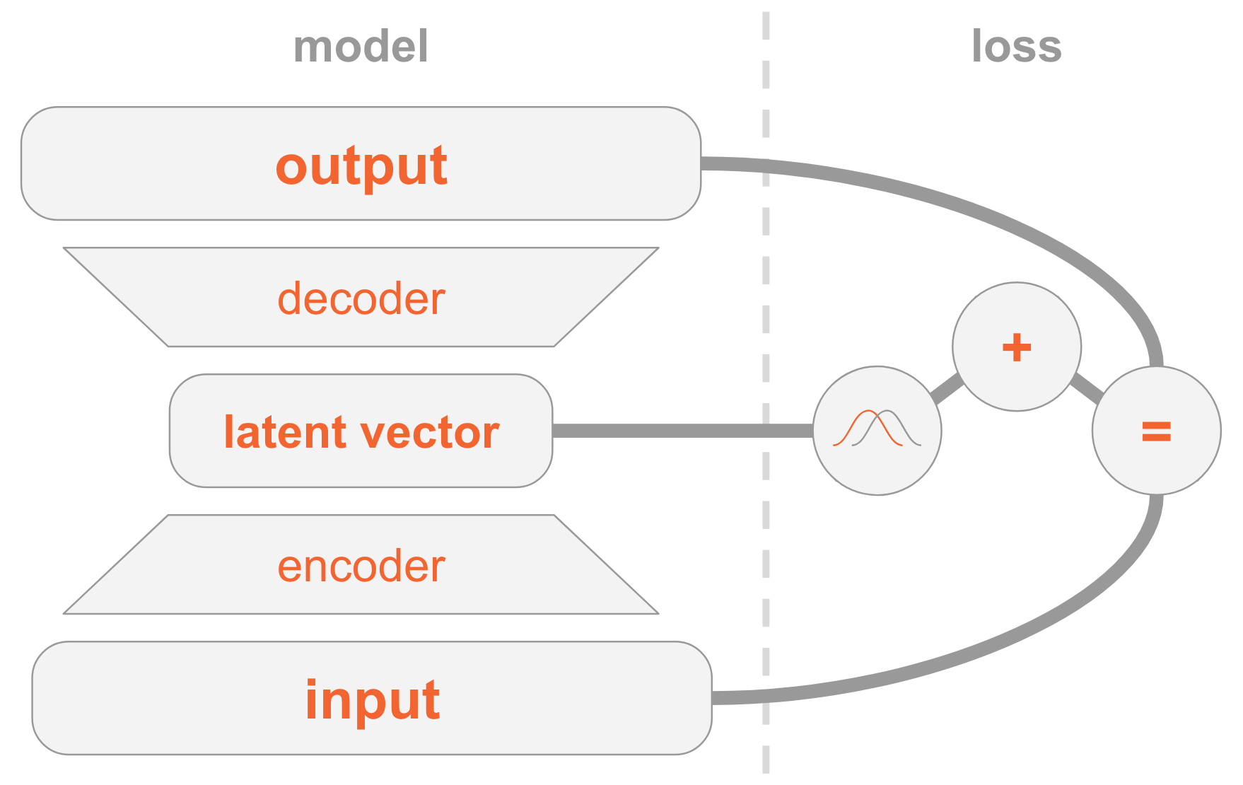
On the left we have the definition of a model:

1. The input image is transmitted through the encoder network.
2. The encoder gives the distribution parameters $$.
3. Hidden vector $$ is taken from $$. If the coder is well trained, then in most cases$$ contain a description $$.
4. Decoder decodes $$ in the image.

On the right side we have a loss function:

1. Recovery error: the output should be similar to the input.
2. $$ should be similar to the previous one, that is, a multidimensional standard normal distribution.

To create new images, you can directly select the hidden vector from the previous distribution and decode it into an image.

Working code

Now let's take a closer look at VAE and look at the working code. You will understand all the technical details necessary for implementing VAE. As a bonus, I will show an interesting trick: how to assign specific roles to some dimensions of the hidden vector so that the model starts generating pictures of the indicated numbers.

import numpy as np
import tensorflow as tf
from tensorflow.examples.tutorials.mnist import input_data
import matplotlib.pyplot as plt
np.random.seed(42)
tf.set_random_seed(42)
%matplotlib inline

I remind you that models are trained on MNIST - a set of handwritten numbers. Input images come in the format$$.

mnist = input_data.read_data_sets('MNIST_data')
input_size = 28 * 28
num_digits = 10

Next, we define the hyperparameters.

Feel free to play with different values ​​to get an idea of ​​how they affect the model.

params = {
    'encoder_layers': [128],                # кодировщик на простой сети прямого распространения'decoder_layers': [128],                # как и декодер (CNN лучше, но не хочу усложнять код)'digit_classification_layers': [128],   # нужно для условий, объясню позже'activation': tf.nn.sigmoid,            # функция активации используется всеми подсетями'decoder_std': 0.5,                     # стандартное отклонение P(x|z) обсуждалось выше'z_dim': 10,                            # размерность скрытого пространства'digit_classification_weight': 10.0,    # нужно для условий, объясню позже'epochs': 20,
    'batch_size': 100,
    'learning_rate': 0.001
}

Model

The model consists of three subnets:

1. Gets $$ (image) encodes it into a distribution $$ on the hidden space.
2. Gets $$ in the hidden space (image code representation), decodes it into the corresponding image $$.
3. Gets $$ and determines the figure in comparison with the 10-dimensional layer, where the i-th value contains the probability of the i-th number.

The first two subnets are the basis of pure VAE.

The third is an auxiliary task that uses some of the hidden dimensions to encode a digit found in an image. Let me explain why: we have previously discussed that we don’t care what information each dimension of hidden space contains. The model can learn to code any information that it considers valuable for its task. Since we are familiar with the data set, we know the importance of a measurement that contains a type of digit (that is, its numerical value). And now we want to help the model by providing it with this information.

Given a type of digit, we directly encode it, that is, we use a vector of size 10. These ten numbers are associated with a hidden vector, so when decoding this vector into an image, the model will use digital information.

There are two ways to provide direct coding vector models:

1. Add it as input to the model.
2. Add it as a label, so the model will calculate the forecast itself: we will add another subnet that predicts a 10-dimensional vector, where the loss function is the cross entropy with the expected direct encoding vector.

Choose the second option. Why? Well, then when testing, you can use the model in two ways:

1. Specify the image as input and display the hidden vector.
2. Specify a hidden vector as input and generate an image.

Since we want to support the first option, we cannot give the model a figure as input, because we do not want to know it during testing. Therefore, the model must learn to predict it.

defencoder(x, layers):for layer in layers:
        x = tf.layers.dense(x,
                            layer,
                            activation=params['activation'])
    mu = tf.layers.dense(x, params['z_dim'])
    var = 1e-5 + tf.exp(tf.layers.dense(x, params['z_dim']))
    return mu, var
defdecoder(z, layers):for layer in layers:
        z = tf.layers.dense(z,
                            layer,
                            activation=params['activation'])
    mu = tf.layers.dense(z, input_size)
    return tf.nn.sigmoid(mu)
defdigit_classifier(x, layers):for layer in layers:
        x = tf.layers.dense(x,
                            layer,
                            activation=params['activation'])
    logits = tf.layers.dense(x, num_digits)
    return logits

images = tf.placeholder(tf.float32, [None, input_size])
digits = tf.placeholder(tf.int32, [None])
# кодируем изображение в распределение по скрытому пространству
encoder_mu, encoder_var = encoder(images,
                                  params['encoder_layers'])
# отбираем вектор из скрытого пространства, используя# трюк с повторной параметризацией
eps = tf.random_normal(shape=[tf.shape(images)[0],
                              params['z_dim']],
                       mean=0.0,
                       stddev=1.0)
z = encoder_mu + tf.sqrt(encoder_var) * eps
# classify the digit
digit_logits = digit_classifier(images,
                                params['digit_classification_layers'])
digit_prob = tf.nn.softmax(digit_logits)
# декодируем в изображение скрытый вектор, связанный# с классификацией цифр
decoded_images = decoder(tf.concat([z, digit_prob], axis=1),
                         params['decoder_layers'])

# потеря состоит в том, насколько хорошо мы # можем восстановить изображение
loss_reconstruction = -tf.reduce_sum(
    tf.contrib.distributions.Normal(
        decoded_images,
        params['decoder_std']
    ).log_prob(images),
    axis=1
)
# и как далеко распределение по скрытому пространству от предыдущего.# Если предыдущее является стандартным гауссовским распределением, # а в результате получается нормальное распределение с диагональной# конвариантной матрицей, то KL-расхождение становится аналитически# разрешимым, и мы получаем
loss_prior = -0.5 * tf.reduce_sum(
    1 + tf.log(encoder_var) - encoder_mu ** 2 - encoder_var,
    axis=1
)
loss_auto_encode = tf.reduce_mean(
    loss_reconstruction + loss_prior,
    axis=0
)
# digit_classification_weight используется как вес между двумя потерями,# поскольку между ними есть напряжение
loss_digit_classifier = params['digit_classification_weight'] * tf.reduce_mean(
    tf.nn.sparse_softmax_cross_entropy_with_logits(labels=digits,
                                                   logits=digit_logits),
    axis=0
)
loss = loss_auto_encode + loss_digit_classifier
train_op = tf.train.AdamOptimizer(params['learning_rate']).minimize(loss)

Training

We will tutor the optimization model of two loss functions - VAE and classification - using SGD .

At the end of each epoch, we select hidden vectors and decode them into images in order to visually observe how the generative power of the model improves according to epochs. The sampling method is as follows:

1. Explicitly specify the dimensions that are used to categorize by the number we want to generate. For example, if we want to create an image of digit 2, then we set measurements$$.
2. Make a random sample from other dimensions of the multidimensional normal distribution. These are the values ​​for the different digits that are generated in a given era. So we get an idea of ​​what is encoded in other dimensions, for example, handwriting style.

The meaning of step 1 is that after convergence, the model should be able to classify a digit in the input image according to these measurement settings. However, they are also used at the decoding stage to create an image. That is, the decoder subnet knows: when the measurements correspond to digit 2, it must generate a picture with this digit. Therefore, if you manually set the measurement to the number 2, we get the generated image of this number.

samples = []
losses_auto_encode = []
losses_digit_classifier = []
with tf.Session() as sess:
    sess.run(tf.global_variables_initializer())
    for epoch in xrange(params['epochs']):
        for _ in xrange(mnist.train.num_examples / params['batch_size']):
            batch_images, batch_digits = mnist.train.next_batch(params['batch_size'])
            sess.run(train_op, feed_dict={images: batch_images, digits: batch_digits})
        train_loss_auto_encode, train_loss_digit_classifier = sess.run(
            [loss_auto_encode, loss_digit_classifier],
            {images: mnist.train.images, digits: mnist.train.labels})
        losses_auto_encode.append(train_loss_auto_encode)
        losses_digit_classifier.append(train_loss_digit_classifier)
        sample_z = np.tile(np.random.randn(1, params['z_dim']), reps=[num_digits, 1])
        gen_samples = sess.run(decoded_images,
                               feed_dict={z: sample_z, digit_prob: np.eye(num_digits)})
        samples.append(gen_samples)

Let's check that both loss functions look good, that is, decrease:

plt.subplot(121)
plt.plot(losses_auto_encode)
plt.title('VAE loss')
plt.subplot(122)
plt.plot(losses_digit_classifier)
plt.title('digit classifier loss')
plt.tight_layout()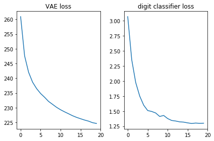

In addition, let's derive the generated images and see if the model is really able to create pictures with handwritten numbers:

defplot_samples(samples):
    IMAGE_WIDTH = 0.7
    plt.figure(figsize=(IMAGE_WIDTH * num_digits,
                        len(samples) * IMAGE_WIDTH))
    for epoch, images in enumerate(samples):
        for digit, image in enumerate(images):
            plt.subplot(len(samples),
                        num_digits,
                        epoch * num_digits + digit + 1)
            plt.imshow(image.reshape((28, 28)),
                       cmap='Greys_r')
            plt.gca().xaxis.set_visible(False)
            if digit == 0:
                plt.gca().yaxis.set_ticks([])
                plt.ylabel('epoch {}'.format(epoch + 1),
                           verticalalignment='center',
                           horizontalalignment='right',
                           rotation=0,
                           fontsize=14)
            else:
                plt.gca().yaxis.set_visible(False)
plot_samples(samples)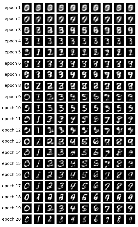

Conclusion

It's nice to see that a simple network of direct distribution (without fancy bundles) generates beautiful images in just 20 epochs. The model quickly learned how to use specific measurements for numbers: in the 9th era, we already see the sequence of numbers that we were trying to generate.

Each epoch used different random values ​​for other dimensions, so the style is different between eras, but similar within them: at least within some. For example, in the 18th all the numbers are fatter compared to the 20th.

Notes

The article is based on my experience and the following sources:

• Variational inference and deep learning: a new synthesis
• Guide to Variational Car Encoders