Machine learning: predict stock prices in the stock market
Translator Polina Kabirova, specifically for Netologiya , adapted the article by Cambridge University engineer Vivek Palaniappan on how to create a model using neural networks that can predict stock prices on the stock exchange.
Machine and deep learning has become a new efficient strategy that many investment funds use to increase revenues. In the article I will explain how neural networks help predict the situation on the stock market - for example, the price of shares (or index). At the heart of the text is my project written in Python. The full code and program guide can be found on GitHub. For more related articles, read the Medium blog .
Changes in finance occur nonlinearly, and sometimes it may seem that stock prices are formed in a completely random fashion. Traditional time series methods such as the ARIMA and GARCH models are effective when the series is stationary — its basic properties do not change over time. And for this, it is necessary that the series be pre-processed with the help
The solution to this problem can be neural networks that do not require stationarity. Neural networks are initially very effective in finding connections between data and are able to predict (or classify) new data based on them.
Usually data science project consists of the following operations:
The input to our neural network is the stock price data for the last 10 days. With their help, we predict prices the next day.
Fortunately, the data required for this project can be found at Yahoo Finance. Data can be collected using their Python API
In our case, the data should be broken down into training sets consisting of 10 past prices and the next day prices. For this, I have defined a class
Similarly, I defined a method that converts test data
For the project, I used two models of neural networks: the Rumelhart Multilayer Perceptron (MLP) and the Long Short Term Model (LSTM) perceptron. Briefly tell about how these models work. Read more about MLP in another article , and about the work of LSTM - in the material by Jacob Aungiers.
MLP is the simplest form of neural networks. The input data gets into the model and with the help of certain weights the values are transmitted through hidden layers to get the output data. The learning algorithm comes from back propagation through hidden layers to change the value of the weights of each neuron. The problem with this model is the lack of “memory”. It is impossible to determine what the previous data was and how they can and should affect the new ones. In the context of our model, 10-day differences between the two datasets may be important, but MLPs are not able to analyze such relationships.
For this, LSTM or Recurrent Neural Networks (RNN) is used. RNNs retain certain information about the data for later use, which helps the neural network to analyze the complex structure of relationships between share price data. But with RNN, a disappearing gradient problem arises. The gradient decreases because the number of layers increases and the level of learning (value less than one) is multiplied several times. Solve this problem LSTM, increasing efficiency.
To implement the model I used
An important stage in dealing with stock prices is data normalization. Usually for this you subtract the average error and divide by the standard error. But we need this system to be used in real trading for a certain period of time. Thus, using statistics may not be the most accurate way to normalize data. Therefore, I simply divided all data into 200 (an arbitrary number, compared to which all other numbers are small). And although it seems that such a normalization is not justified by anything and does not make sense, it is effective to make sure that the weights in the neural network do not become too large.
Let's start with a simpler model - MLP. In Keras, a sequence is built and dense layers are added on top of it. The full code looks like this:
Using Keras in five lines of code, we created MLPs with hidden layers, one hundred neurons each. And now a little about the optimizer. The Adam (adaptive moment estimation) method is gaining popularity. It is a more efficient optimization algorithm compared to stochastic gradient descent . There are two other extensions of the stochastic gradient descent - the Adam advantages are immediately visible against their background:
AdaGrad supports the established learning speed, which improves the results when gradients differ (for example, problems with natural language and computer vision).
Rmsprop- supports the established learning rate, which may vary depending on the average values of recent gradients for weight (for example, how quickly it changes). This means that the algorithm copes well with unsteady problems (for example, noise).
Adam combines the benefits of these extensions, so I chose it.
Now we customize the model to our training data. Keras simplifies the task again, only the following code is needed:
When the model is ready, you need to test it on test data to determine how well it worked. This is done like this:
Information obtained as a result of the test can be used to evaluate the model's ability to predict stock prices.
A similar procedure is used for the LSTM model, so I will show the code and explain it a little:
Please note that Keras needs data of a certain size, depending on your model. It is very important to change the shape of the array with NumPy.
When we have prepared our models with the help of training data and tested them on test data, we can test the model on historical data. This is done as follows:
However, this is a simplified version of testing. For a complete backtesting system, factors such as “survival error” (survivorship bias), tendentiousness (look ahead bias), changing market conditions and transaction costs should be taken into account. Since this is just an educational project, there is enough back-testing.
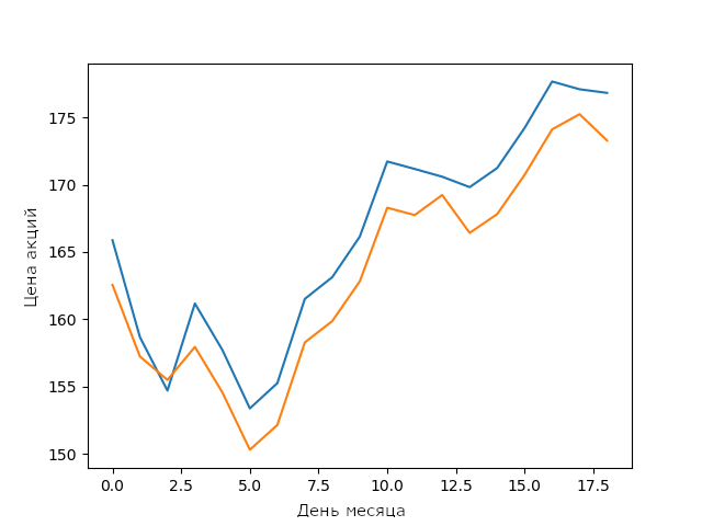
The forecast of my LSTM model for Apple stock prices in February
For a simple LSTM model without optimization, this is a very good result. It shows that neural networks and machine learning models are capable of building complex stable connections between parameters.
To improve model results after testing, optimization is often needed. I did not include it in the open source version so that readers can try to optimize the model themselves. Those who do not know how to optimize will have to find hyper parameters that will improve the performance of the model. There are several methods for searching hyper parameters: from the selection of parameters by the grid to stochastic methods.
I am confident that with the optimization of models of knowledge in the field of machine learning, they are reaching a new level. Try to optimize the model so that it works better than mine. Compare the result with the schedule above.
Machine learning is constantly evolving - new methods are emerging every day, so it is very important to constantly learn. The best way to do this is to create interesting projects, for example, to build models for predicting stock prices. And although my LSTM model is not good enough for use in real trading, the foundation laid in developing such a model may help in the future.
Courses "Netology" on the topic:
Machine and deep learning has become a new efficient strategy that many investment funds use to increase revenues. In the article I will explain how neural networks help predict the situation on the stock market - for example, the price of shares (or index). At the heart of the text is my project written in Python. The full code and program guide can be found on GitHub. For more related articles, read the Medium blog .
Neural networks in economics
Changes in finance occur nonlinearly, and sometimes it may seem that stock prices are formed in a completely random fashion. Traditional time series methods such as the ARIMA and GARCH models are effective when the series is stationary — its basic properties do not change over time. And for this, it is necessary that the series be pre-processed with the help
log returnsor brought to stationarity differently. However, the main problem arises when these models are implemented in a real trading system, since when adding new data stationarity is not guaranteed. The solution to this problem can be neural networks that do not require stationarity. Neural networks are initially very effective in finding connections between data and are able to predict (or classify) new data based on them.
Usually data science project consists of the following operations:
- Data collection - provides a set of necessary properties.
- Preliminary data processing is often a frightening, but necessary step before using data.
- Development and implementation of the model - the choice of the type of neural network and its parameters.
- Backtesting models (testing on historical data) are the key step of any trading strategy.
- Optimization - search for suitable parameters.
The input to our neural network is the stock price data for the last 10 days. With their help, we predict prices the next day.
Data collection
Fortunately, the data required for this project can be found at Yahoo Finance. Data can be collected using their Python API
pdr.get_yahoo_data(ticker, start_date, end_date)or directly from the site.Preliminary data processing
In our case, the data should be broken down into training sets consisting of 10 past prices and the next day prices. For this, I have defined a class
Preprocessingthat will work with training and test data. Inside the class, I defined a method get_train(self, seq_len)that converts the training input and output data into NumPyarrays, specifying a specific window length (in our case 10). All code looks like this:defgen_train(self, seq_len):
"""
Generates training data
:param seq_len: length of window
:return: X_train and Y_train
"""
for i in range((len(self.stock_train)//seq_len)*seq_len - seq_len - 1):
x = np.array(self.stock_train.iloc[i: i + seq_len, 1])
y = np.array([self.stock_train.iloc[i + seq_len + 1, 1]], np.float64)
self.input_train.append(x)
self.output_train.append(y)
self.X_train = np.array(self.input_train)
self.Y_train = np.array(self.output_train)Similarly, I defined a method that converts test data
X_testand Y_test.Neural network models
For the project, I used two models of neural networks: the Rumelhart Multilayer Perceptron (MLP) and the Long Short Term Model (LSTM) perceptron. Briefly tell about how these models work. Read more about MLP in another article , and about the work of LSTM - in the material by Jacob Aungiers.
MLP is the simplest form of neural networks. The input data gets into the model and with the help of certain weights the values are transmitted through hidden layers to get the output data. The learning algorithm comes from back propagation through hidden layers to change the value of the weights of each neuron. The problem with this model is the lack of “memory”. It is impossible to determine what the previous data was and how they can and should affect the new ones. In the context of our model, 10-day differences between the two datasets may be important, but MLPs are not able to analyze such relationships.
For this, LSTM or Recurrent Neural Networks (RNN) is used. RNNs retain certain information about the data for later use, which helps the neural network to analyze the complex structure of relationships between share price data. But with RNN, a disappearing gradient problem arises. The gradient decreases because the number of layers increases and the level of learning (value less than one) is multiplied several times. Solve this problem LSTM, increasing efficiency.
Model implementation
To implement the model I used
Keras, because there the layers are added gradually, and do not define the entire network at once. So we can quickly change the number and type of layers, optimizing the neural network.An important stage in dealing with stock prices is data normalization. Usually for this you subtract the average error and divide by the standard error. But we need this system to be used in real trading for a certain period of time. Thus, using statistics may not be the most accurate way to normalize data. Therefore, I simply divided all data into 200 (an arbitrary number, compared to which all other numbers are small). And although it seems that such a normalization is not justified by anything and does not make sense, it is effective to make sure that the weights in the neural network do not become too large.
Let's start with a simpler model - MLP. In Keras, a sequence is built and dense layers are added on top of it. The full code looks like this:
model = tf.keras.models.Sequential()
model.add(tf.keras.layers.Dense(100, activation=tf.nn.relu))
model.add(tf.keras.layers.Dense(100, activation=tf.nn.relu))
model.add(tf.keras.layers.Dense(1, activation=tf.nn.relu))
model.compile(optimizer="adam", loss="mean_squared_error")
Using Keras in five lines of code, we created MLPs with hidden layers, one hundred neurons each. And now a little about the optimizer. The Adam (adaptive moment estimation) method is gaining popularity. It is a more efficient optimization algorithm compared to stochastic gradient descent . There are two other extensions of the stochastic gradient descent - the Adam advantages are immediately visible against their background:
AdaGrad supports the established learning speed, which improves the results when gradients differ (for example, problems with natural language and computer vision).
Rmsprop- supports the established learning rate, which may vary depending on the average values of recent gradients for weight (for example, how quickly it changes). This means that the algorithm copes well with unsteady problems (for example, noise).
Adam combines the benefits of these extensions, so I chose it.
Now we customize the model to our training data. Keras simplifies the task again, only the following code is needed:
model.fit(X_train, Y_train, epochs=100)When the model is ready, you need to test it on test data to determine how well it worked. This is done like this:
model.evaluate(X_test, Y_test)Information obtained as a result of the test can be used to evaluate the model's ability to predict stock prices.
A similar procedure is used for the LSTM model, so I will show the code and explain it a little:
model = tf.keras.Sequential()
model.add(tf.keras.layers.LSTM(20, input_shape=(10, 1), return_sequences=True))
model.add(tf.keras.layers.LSTM(20))
model.add(tf.keras.layers.Dense(1, activation=tf.nn.relu))
model.compile(optimizer="adam", loss="mean_squared_error")
model.fit(X_train, Y_train, epochs=50)
model.evaluate(X_test, Y_test)
Please note that Keras needs data of a certain size, depending on your model. It is very important to change the shape of the array with NumPy.
Backtesting models
When we have prepared our models with the help of training data and tested them on test data, we can test the model on historical data. This is done as follows:
defback_test(strategy, seq_len, ticker, start_date, end_date, dim):
   """
   A simple back test for a given date period
   :param strategy: the chosen strategy. Note to have already formed the model, and fitted with training data.
   :param seq_len: length of the days used for prediction
   :param ticker: company ticker
   :param start_date: starting date
   :type start_date: "YYYY-mm-dd"
   :param end_date: ending date
   :type end_date: "YYYY-mm-dd"
   :param dim: dimension required for strategy: 3dim for LSTM and 2dim for MLP
   :type dim: tuple
   :return: Percentage errors array that gives the errors for every test in the given date range
   """
   data = pdr.get_data_yahoo(ticker, start_date, end_date)
   stock_data = data["Adj Close"]
   errors = []
   for i in range((len(stock_data)//10)*10 - seq_len - 1):
       x = np.array(stock_data.iloc[i: i + seq_len, 1]).reshape(dim) / 200
       y = np.array(stock_data.iloc[i + seq_len + 1, 1]) / 200
       predict = strategy.predict(x)
       while predict == 0:
           predict = strategy.predict(x)
       error = (predict - y) / 100
       errors.append(error)
       total_error = np.array(errors)
   print(f"Average error = {total_error.mean()}")
However, this is a simplified version of testing. For a complete backtesting system, factors such as “survival error” (survivorship bias), tendentiousness (look ahead bias), changing market conditions and transaction costs should be taken into account. Since this is just an educational project, there is enough back-testing.
The forecast of my LSTM model for Apple stock prices in February
For a simple LSTM model without optimization, this is a very good result. It shows that neural networks and machine learning models are capable of building complex stable connections between parameters.
Hyperparameter Optimization
To improve model results after testing, optimization is often needed. I did not include it in the open source version so that readers can try to optimize the model themselves. Those who do not know how to optimize will have to find hyper parameters that will improve the performance of the model. There are several methods for searching hyper parameters: from the selection of parameters by the grid to stochastic methods.
I am confident that with the optimization of models of knowledge in the field of machine learning, they are reaching a new level. Try to optimize the model so that it works better than mine. Compare the result with the schedule above.
Conclusion
Machine learning is constantly evolving - new methods are emerging every day, so it is very important to constantly learn. The best way to do this is to create interesting projects, for example, to build models for predicting stock prices. And although my LSTM model is not good enough for use in real trading, the foundation laid in developing such a model may help in the future.
From the Editor
Courses "Netology" on the topic:
- online profession " Data Analyst "
- online profession " Data Scientist "