Prelude

Numerical solution of linear systems of equations is an indispensable step in many areas of applied mathematics, engineering and IT-industry, whether it is working with graphics, calculating the aerodynamics of any aircraft or optimizing logistics. Fashionable now "machine" without this, too, would not really progressed. Moreover, the solution of linear systems, as a rule, consumes the largest percentage of all computational costs. It is clear that this critical component requires maximum speed optimization.

Often work with the so-called. sparse matrices - those with zeros by orders of magnitude more than other values. This, for example, is inevitable if you deal with equations in partial derivatives or with any other processes in which the elements that arise in the defining linear relations are associated only with "neighbors". Here is a possible example of a sparse matrix for the one-dimensional Poisson equation known in classical physics.$$ on a uniform grid (yes, as long as there are not so many zeros in it, but when grinding the grid, they will be healthy!):

$$

The matrices opposite to them — those in which the number of zeros is not paid attention to and take into account all components without exception — are called dense.

Sparse matrices are often, for various reasons, presented in a compressed columnar format - Compressed Sparse Column (CSC). In this description, two integer arrays and one with a floating point are used. Let the matrix have$$ nonzero and $$columns. Elements of the matrix are listed in columns from left to right, with no exceptions. First array$$ lengths $$contains the row numbers of nonzero matrix components. Second array$$ lengths $$contains ... no, not column numbers, because then the matrix would be written in the coordinate format (coordinate), or triplet. And the second array contains the ordinal numbers of those components of the matrix, from which the columns begin, including an additional dummy column at the end. Finally, the third array$$ lengths $$already contains the components themselves, in the order corresponding to the first array. Here, for example, assuming that the numbering of rows and columns of matrices starts from zero, for a specific matrix

$$

arrays will be $$, $$, $$.

Methods for solving linear systems are divided into two large classes - direct and iterative. Straight lines are based on the ability to represent the matrix as a product of two simpler matrices, in order to split the solution into two simple steps. Iteration uses the unique properties of linear spaces and works on the ancient as the world method of consistent approximation of the unknowns to the desired solution, and in the process of convergence of the matrix are used, as a rule, only to multiply them by vectors. Iterative methods are much cheaper than direct ones, but sluggishly work on ill-conditioned matrices. When reinforced concrete reliability is important - use straight lines. Here I want to touch them a little.

Let's say for a square matrix$$ we have the decomposition of the form $$where $$ and $$- respectively, the lower triangular and upper triangular matrices, respectively. The first means that it has one zeros above the diagonal, the second - that it is lower than the diagonal. How exactly we got this decomposition - we are not interested. Here is a simple decomposition example:

$$

How in this case to solve the system of equations $$for example with the right side $$? The first stage is a forward move (forward solve = forward substitution). Denote$$ and work with the system $$. Since$$ - lower triangular, successively in the cycle we find all the components $$ top down:

$$

The central idea is that, by finding $$vector components $$, it is multiplied by a column with the same matrix number $$which is then subtracted from the right side. The matrix itself seems to collapse from left to right, decreasing in size as more and more components of the vector are found.$$. This process is called “column destruction”.

The second stage is reverse (backward solve = backward substitution). Having found a vector$$decide $$. Here we are already going to components from the bottom up, but the idea remains the same:$$column is multiplied by the component just found $$and is transferred to the right, and the matrix collapses from right to left. The whole process is illustrated for the matrix mentioned in the example in the picture below:

$$

$$

and our decision will be $$.

If the matrix is ​​dense, that is, it is fully represented as an array, one-dimensional or two-dimensional, and access to a specific element in it occurs during$$, then a similar solution procedure with the already existing decomposition is not difficult and is coded easily, so we will not even spend time on it. What if the matrix is ​​sparse? Here, in principle, is also not difficult. Here is the C ++ code for the direct move, in which the solution$$written for the place of the right-hand side, without validating the input data (CSC arrays correspond to the lower triangular matrix):

Algorithm 1:

voidforward_solve(conststd::vector<size_t>& iA, conststd::vector<size_t>& jA, conststd::vector<double>& vA, std::vector<double>& x){
    size_t j, p, n = x.size();
    for (j = 0; j < n; j++) // цикл по столбцам
    {
        x[j] /= vA[jA[j]];
        for (p = jA[j]+1; p < jA[j+1]; p++)
            x[iA[p]] -= vA[p] * x[j] ;
    }
}

All further discussion will concern only the direct course for solving the lower triangular system. $$.

Outset

And what if the right side, i.e. vector to the right of the equal sign$$, itself has a large number of zeros? Then it makes sense to skip the calculations associated with zero positions. Changes in the code in this case are minimal:

Algorithm 2:

voidfake_sparse_forward_solve(conststd::vector<size_t>& iA, conststd::vector<size_t>& jA, conststd::vector<double>& vA, std::vector<double>& x){
    size_t j, p, n = x.size();
    for (j = 0; j < n; j++) // цикл по столбцам
    {
        if(x[j])
        {
            x[j] /= vA[jA [j]];
            for (p = jA[j]+1; p < jA[j+1]; p++)
                x[iA[p]] -= vA[p] * x[j];
        }
    }
}

The only thing we added is an operator ifwhose goal is to reduce the number of arithmetic operations to their actual number. If, for example, the entire right-hand side consists of zeros, then nothing should be considered: the decision will be the right-hand side.

Everything looks great and of course it will work, but here, after a long prelude, the problem is finally visible - the asymptotically poor performance of this solver in the case of large systems. And all because of the very fact of having a cycle for. What is the problem? Even if the condition inside ifis true very rarely, one cannot get away from the cycle itself, and this causes the complexity of the algorithm$$where $$- the size of the matrix. No matter how the cycles are optimized by modern compilers, this complexity will make itself felt at large$$. Especially sad when the whole vector$$entirely consists of zeros, because, as we said, and in this case, then do nothing! Not a single arithmetic operation! What the hell$$action?

Well, let's say. Even if so, why not just endure a run forat idle, because of real calculations with real numbers, i.e. those that fall under if, will still be small? But the fact is that this procedure of a forward stroke with a sparse right-hand side itself is often used in external cycles and underlies the Cholesky decomposition.$$and left-looking LU decomposition . Yes, one of those expansions, without the ability to make all these direct and reverse moves in solving linear systems lose all practical meaning.

Theorem. If the matrix is ​​symmetric positive-definite (SPD), then it can be represented as$$ the only way where $$- lower triangular matrix with positive elements on the diagonal.

For highly sparse SPD matrices, a Cholesky decomposition is used. Schematically representing decomposition in a matrix-block form

$$

The whole factorization process can be logically divided into just three steps.

Algorithm 3:

1. lower cholesky decomposition method $$ (recursion!)
2. lower triangular system with sparse right side $$( here it is! )
3. calculation $$ (trivial operation)

In practice, this is implemented in such a way that in one large cycle, steps 3 and 2 are performed, and in that order. Thus, the matrix is ​​run diagonally from top to bottom, increasing the matrix$$line by line on each iteration of the loop.

If in a similar aglorythm the difficulty of a forward move in step 2 is$$where $$ - the size of the lower triangular matrix $$ on an arbitrary iteration of a large cycle, the complexity of the entire decomposition will be at least $$! Oh, how it would not like!

State of the art

Many algorithms are somehow based on the mimicking of human actions in solving problems. If we give a person a lower-triangular linear system with the right side, in which only 1-2 are nonzero, then he will first, of course, run the vector of the right side with eyes from top to bottom$$! ) to find these nonuli. Then he will use them only, without wasting time on zero components, because the solutions will not affect the solution: there is no point in dividing zeros into diagonal components of the matrix, as well as moving the column multiplied by zero to the right. This is the algorithm shown above 2. There are no miracles. But what if a person is immediately given non-zero component numbers from some other sources? For example, if the right-hand side is a column of some other matrix, as is the case with the Cholesky decomposition, then we have instant access to its non-zero components if we request them sequentially:

// если столбец с индексом j, то пробегаем только ненулевые элементы:for (size_t p = jA[j]; p < jA[j+1]; p++)
// получаем ненулевой элемент vA[p] матрицы на пересечении строки iA[p] и столбца j

The difficulty of such access is $$where $$- the number of nonzero components in column j. Thank God for the CSC format! As you can see, it is not only used to save memory.

In this case, we can catch the very essence of what is happening when solving by the method of a forward move$$ for sparse matrix $$ and the right side $$. Hold your breath: we take a non-zero component$$ in the right part, we find the corresponding variable $$ by dividing by $$and then, multiplying the entire i-th column by this found variable, we introduce additional non-nulls in the right-hand side by subtracting this column from the right-hand side! This process is perfectly described in the language of ... graphs. Moreover, oriented and non-cyclical.

We define for a lower triangular matrix that has no zeros on the diagonal, a connected graph. We assume that the numbering of rows and columns starts from zero.
Definition Connectivity graph for a lower triangular matrix$$ size $$which has no zeros on the diagonal, let's call the set of nodes $$ and oriented edges $$.

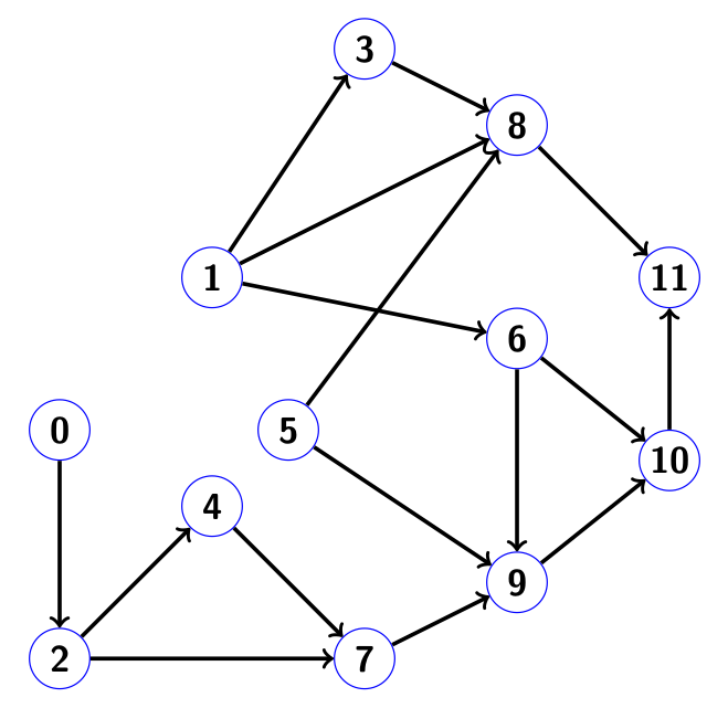
Here, for example, looks like a connectivity graph for a lower triangular matrix.

in which the numbers simply correspond to the ordinal number of the diagonal element, and the dots denote nonzero components below the diagonal:



Definition Reachability of a directed graph$$ on a set of indices $$ let's call such a set of indices $$that in any index $$ You can get to the passage on the graph with some index $$.

Example: for the graph from the image$$. Clear that always runs$$.

If we represent each node of the graph as the column number of the matrix that generated it, the neighboring nodes, to which its edges are directed, correspond to the row numbers of the nonzero components in this column.

Let be$$denotes a set of indices corresponding to nonzero positions in the vector x.

Hubert's theorem (no, not the one whose name the spaces are named) Set$$where $$ there is a solution vector of a rarefied lower triangular system $$ with sparse right side $$, coincides with $$.

Addition from ourselves: in the theorem we do not take into account the unlikely possibility that non-zero numbers on the right-hand side, when killing columns, can be reduced to zero, for example, 3 - 3 = 0. This effect is called numerical cancellation. To take into account such spontaneously occurring zeros is a waste of time, and they are perceived like all other numbers in non-zero positions.

The effective method of carrying out a direct stroke with a given sparse right-hand side, assuming that we have direct access to its non-zero components by index, is as follows.

1. It is run by Earl " dfs " (depth first search), sequentially starting from the index$$every nonzero component of the right side. Write found nodes to array$$at the same time we perform in the order in which we return back in the graph! By analogy with the army of invaders: we occupy the country without cruelty, but when we began to drive back, we are angry, we destroy everything in our path.
   It is worth noting that it is absolutely not necessary that the list of indexes$$It was sorted by rerun when it was fed to the input of the "depth-first search" algorithm. You can start in any order on the set$$. Different ordering of belonging to the set$$indexes does not affect the final decision, as we will see in the example.
   
   This step does not require any knowledge of the real array at all.$$! Welcome to the world of symbolic analysis when working with direct sparse solvers!
   
2. We proceed to the solution itself, having at its disposal an array $$from the previous step. Columns are destroyed in the reverse order of the record of this array . Voila!

Example

Consider an example in which both steps are shown in detail. Suppose we have a matrix of size 12 x 12 of the following form:

The corresponding connectivity graph has the form:

Let the right side of nonuli are only at positions 3 and 5, that is, $$. Let's run the graph, starting from these indices in the written order. Then the “depth-first search” method will look as follows. First we will visit the indexes in order.$$, not forgetting to mark the indexes as visited. In the image below they are painted in blue:

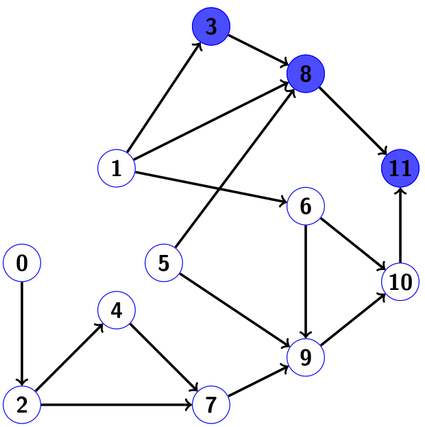
When going back, we put the indices into our array of indices of nonzero components of the solution. $$. Next, try to run$$, but we come across the already marked node 8, so we don’t touch this route and proceed to the branch $$. The result of this run will be$$. Site 11 can not visit, since it is already labeled. So, go back and complete the array$$ New catch marked in green: $$. And here is the drawing:

Cloudy green nodes 8 and 11 are those that we wanted to visit during the second run, but could not, because already visited during the first.

So the array$$formed. Go to the second step. A simple step: run through the array$$ in the reverse order (right to left), finding the corresponding components of the solution vector $$ dividing by the diagonal components of the matrix $$and moving the columns to the right. The remaining components$$as they were zeros, they remained so. Schematically, this is shown below, where the bottom arrow indicates the order in which columns are destroyed:

Please note: in this order, the destruction of columns number 3 will meet later numbers 5, 9 and 10! Columns are not destroyed in an order sorted in ascending order, which would be a mistake for dense ones, i.e. unbreakable matrices. But for sparse matrices like in the order of things. As can be seen from the non-zero structure of the matrix in this example, the use of columns 5, 9 and 10 to column 3 will not distort the components in the answer.$$, $$, $$ not at all, they have c $$just "no intersection." Our method took it into account! Similarly, using column 8 after column 9 will not spoil a component.$$. Excellent algorithm, is not it?

If we go around the graph from index 5 first, and then from index 3, then our array will be$$. Destroying the columns in the reverse order of this array will give exactly the same solution as in the first case!

The complexity of all our operations is scaled according to the number of actual arithmetic operations and the number of nonzero components on the right side, but not the size of the matrix! We have achieved our goal.

Criticism

BUT! A critical reader will notice that the very assumption at the beginning, as if we have “direct access to non-zero components of the right part by indices,” already means that once we ran the right part from top to bottom to find these indices in the array$$that is already spent $$action! Moreover, the graph's mileage itself requires that we pre-allocate the memory of the maximum possible length (we need to write down the indexes found by the search in depth!), So as not to suffer with further relocation as the array grows$$This also requires $$operations! Why then, they say, all the fuss?

But indeed, for a one-time solution of a sparse lower triangular system with a sparse right-hand side, initially given as a dense vector, there is no point in wasting developer time on all the above-mentioned algorithms. They may be even slower than the method in the forehead, represented by algorithm 2 above. But, as mentioned earlier, this device is indispensable for Cholesky factorization, so you should not throw tomatoes at me. Indeed, before running algorithm 3, all the necessary memory of maximum length is allocated immediately and requires$$of time. In the subsequent cycle in columns$$ all data is only overwritten in a fixed-length array $$, and only in those positions in which this perezapist actual, thanks to direct access to nonzero elements. And it is precisely due to this that efficiency arises!

C ++ implementation

The graph itself as a data structure in the code is not necessary to build. It is enough to use it implicitly when working with the matrix directly. All the required connectivity will be taken into account by the algorithm. Search in depth of course convenient to implement using a banal recursion. Here, for example, looks like a recursive depth search based on a single starting index:

/*
j - стартовый индекс
iA, jA - целочисленные массивы нижнетреугольной матрицы, представленной в формате CSC
top - значение текущей глубины массива nnz(x); в самом начале передаём 0
result - массив длины N, на выходе содержит nnz(x) с индекса 0 до top-1 включительно
marked - массив меток длины N; на вход подаём заполненным нулями
*/voidDepthFirstSearch(size_t j, conststd::vector<size_t>& iA, conststd::vector<size_t>& jA, size_t& top, std::vector<size_t>& result, std::vector<int>& marked){
    size_t p;
    marked[j] = 1; // помечаем узел j как посещённыйfor (p = jA[j]; p < jA[j+1]; p++) // для каждого ненулевого элемента в столбце j
    {
        if (!marked[iA[p]]) // если iA[p] не помечен
        {
            DepthFirstSearch(iA[p], iA, jA, top, result, marked); // Поиск в глубину на индексе iA[p]
        }
    }
    result[top++] = j; // записываем j в массив nnz(x)
}

If in the very first call the DepthFirstSearchvariable is transferred topto zero, then after the completion of the entire recursive procedure, the variable topwill be equal to the number of indexes found in the array result. Homework: write another function that accepts an array of indices of nonzero components on the right side and sequentially passes their functions DepthFirstSearch. Without this, the algoryth is not complete. Note: an array of real numbers$$we do not pass to the function at all, since it is not needed in the process of symbolic analysis.

Despite the simplicity, the implementation defect is obvious: for large systems, the stack overflow is not far off. Well then, there is an option based on a cycle instead of recursion. It is more difficult to understand, but already suitable for all occasions:

/*
j - стартовый индекс
N - размер матрицы
iA, jA - целочисленные массивы нижнетреугольной матрицы, представленной в формате CSC
top - значение текущей глубины массива nnz(x)
result - массив длины N, на выходе содержит часть nnz(x) с индексов top до ret-1 включительно, где ret - возвращаемое значение функции
marked - массив меток длины N
work_stack - вспомогательный рабочий массив длины N
*/size_t DepthFirstSearch(size_t j, size_t N, conststd::vector<size_t>& iA, conststd::vector<size_t>& jA, size_t top, std::vector<size_t>& result, std::vector<int>& marked, std::vector<size_t>& work_stack)
{
    size_t p, head = N - 1;
    int done;
    result[N - 1] = j; // инициализируем рекурсионный стекwhile (head < N)
    {
        j = result[head]; // получаем j с верхушки рекурсионного стекаif (!marked[j])
        {
            marked[j] = 1; // помечаем узел j как посещённый
            work_stack[head] = jA[j];
        }
        done = 1; // покончили с узлом j в случае отсутствия непосещённых соседейfor (p = work_stack[head] + 1; p < jA[j+1]; p++) // исследуем всех соседей j
        {
            // работаем с cоседом с номером iA[p]if (marked[iA[p]]) continue; // узел iA[p] посетили раньше, поэтому пропускаем
            work_stack[head] = p; // ставим на паузу поиск по узлу j
            result[--head] = iA[p]; // запускаем поиск в глубину на узле iA[p]
            done = 0; // с узлом j ещё не покончилиbreak;
        }
        if (done) // поиск в глубину на узле j закончен
        {
            head++; // удаляем j из рекурсионного стека
            result[top++] = j; // помещаем j в выходной массив
        }
    }
    return (top);
}

And this is how the generator of a non-zero solution vector structure looks like $$:

/*
iA, jA - целочисленные массивы матрицы, представленной в формате CSC
iF - массив индексов ненулевых компонент вектора правой части f
nnzf - количество ненулей в правой части f
result - массив длины N, на выходе содержит nnz(x) с индексов 0 до ret-1 включительно, где ret - возвращаемое значение функции
marked - массив меток длины N, передаём заполненным нулями
work_stack - вспомогательный рабочий массив длины N
*/size_t NnzX(conststd::vector<size_t>& iA, conststd::vector<size_t>& jA, conststd::vector<size_t>& iF,  size_t nnzf, std::vector<size_t>& result, std::vector<int>& marked, std::vector<size_t>& work_stack)
{
    size_t p, N, top;
    N = jA.size() - 1;
    top = 0;
    for (p = 0; p < nnzf; p++)
        if (!marked[iF[p]]) // начинаем поиск в глубину на непомеченном узле
            top = DepthFirstSearch(iF[p], N, iA, jA, vA, top, result, marked, work_stack);
    for (p = 0; p < top; p++)
        marked[result[p]] = 0; // очищаем меткиreturn (top);
}

Finally, combining everything into one, we write the lower triangular solver itself for the case of a sparse right side:

/*
iA, jA, vA - массивы матрицы, представленной в формате CSC
iF - массив индексов ненулевых компонент вектора правой части f
nnzf - количество ненулей в правой части f
vF - массив ненулевых компонент вектора правой части f
result - массив длины N, на выходе содержит nnz(x) с индексов 0 до ret-1 включительно, где ret - возвращаемое значение функции
marked - массив меток длины N, передаём заполненным нулями
work_stack - вспомогательный рабочий массив длины N
x - вектор решения длины N, которое получим на выходе; на входе заполнен нулями
*/size_t lower_triangular_solve (conststd::vector<size_t>& iA, conststd::vector<size_t>& jA, conststd::vector<double>& vA, conststd::vector<size_t>& iF,  size_t nnzf, conststd::vector<double>& vF, std::vector<size_t>& result, std::vector<int>& marked, std::vector<size_t>& work_stack, std::vector<double>& x)
{
    size_t top, p, j;
    ptrdiff_t px;
    top = NnzX(iA, jA, iF, nnzf, result, marked, work_stack);
    for (p = 0; p < nnzf; p++) x[iF[p]] = vF[p]; // заполняем плотный векторfor (px = top; px > -1; px--) // прогон в обратном порядке
    {
        j = result[px]; // x(j) будет ненулём
        x [j] /= vA[jA[j]]; // мгновенное нахождение x(j)for (p = jA[j]+1; p < jA[j+1]; p++)
        {
            x[iA[p]] -= vA[p]*x[j]; // уничтожение j-ого столбца
        }
    }
    return (top) ;
}

We see that our cycle runs only on the array indices $$rather than the whole set $$. Done!

There is an implementation that does not use an array of tags markedto save memory. Instead, an additional set of indexes is used.$$not intersecting with the set $$in which a one-to-one mapping occurs by a simple algebraic operation as a procedure for marking a node. However, in our era of cheap memory, save it on a single array of length$$ it seems completely redundant.

As a conclusion

The process of solving a rarefied linear equation system by the direct method, as a rule, is divided into three stages:

1. Character analysis
2. Numerical factorization based on solon analysis
3. The solution of the obtained triangular systems with dense right side

The second step, numerical factorization, is the most resource-intensive part and devours most (> 90%) of the estimated time. The purpose of the first step is to reduce the high cost of the second. An example of symbolic analysis was presented in this post. However, it is the first step that requires the longest development time and maximum mental costs on the part of the developer. A good symbolic analysis requires knowledge of the theory of graphs and trees and the possession of an “algorithmic flair”. The second step is disproportionately easier to implement.
Well, the third step and the implementation, and the estimated time in most cases the most unassuming.

A good introduction to direct methods for sparse systems is in the book by Tim Avis , a professor at the faculty of computer science at the University of Texas A & M ,Direct Methods for Sparse Linear Systems ". The algorithm described above is described there. I am not familiar with Davis himself, although I myself once worked at the same university (albeit in another department). If I am not mistaken, Davis himself participated in the development of solvers used in Matlab (!). Moreover, he is involved even in Google Street View image generator (least squares method). By the way, in the same faculty none other than Bjorn Straustrup himself is the creator of the C ++ language.

Maybe someday I'll write something else about sparse matrices or numerical methods in In general, all good!