Coding and testing kNN in Julia

New language in Data Science. In Russia, Julia is a rather rare language, although it has been used abroad for 5 years already (I was also surprised). There are no sources in Russian, so I decided to make an illustrative example of the work of Julia, taken from one wonderful book. The best way to learn a language is to write something on it. And so that it also attracted attention, use machine learning.

Hello Habrozhitelyami.

Some time ago I began to learn a new language Julia. Well, like new. This is something between Matlab and Python, the syntax is very similar, and the language itself is written in C / C ++. In general, the history of creation, what, why and why is on Wikipedia and in a couple of articles on Habré.

The first thing that started my language study was right, I naguglitla Coursera online course in English. There about the basic syntax + in parallel is written a mini-project on the prediction of diseases in Africa. Basics and immediately practice. If you need a certificate, buy the full version. I was free. The difference of this version is that no one will check your tests and DM. It was more important for me to get familiarization than a certificate. (Read clamped 50 bucks)

After I decided that I should read a book on Julia. Google issued a list of books and further studying reviews and reviews, chose one of them and ordered it on Amazon. Book versions are always more pleasant to read and crayon in them.

The book is called Julia for Data Science , by Zacharias Voulgaris, PhD. That excerpt, which I want to submit, contains many typos in the code, which I corrected and therefore present the working version + my results.

kNN

This is an example of the application of the algorithm of classification of the method of nearest neighbors. Probably one of the oldest machine learning algorithms. The algorithm does not have a learning phase and is also quite fast. Its meaning is quite simple: to classify a new object, you need to find similar “neighbors” from the data set (base) and then determine the class by voting.

I’ll make a reservation right now that there are ready-made packages in Julia, and it’s better to use them to reduce time and reduce errors. But this code is, in some way, indicative of the Julia syntax. It is more convenient for me to learn a new language in examples, rather than reading the dry excerpts of the general form of a particular function.

So, what we have at the input:

Training data X (training sample), training data labels x (corresponding tags),testing data Y (test sample), number of neighbors k (number of neighbors).

Three functions will be needed: distance calculation function, classification function and main .

The essence is this: we take one element of the test array, we calculate the distances from it to the elements of the training array. Then we select the indices of those k elements that turned out to be as close as possible. The test element is assigned to the class that is the most common among the k nearest neighbors.

functionCalculateDistance{T<:Number}(x::Array{T,1}, y::Array{T,1})
    dist = 0fori in 1:length(x)
        dist += (x[i] - y[i])^2end
    dist = sqrt(dist)
    return dist
end

The main function of the algorithm. At the entrance comes a matrix of distances between the objects of the training and test sample, the tags of the training sample, the number of the nearest "neighbors". The output predicted labels for new objects and the likelihood of each label.

function Classify{T<:Any}(distances::Array{Float64,1}, labels::Array{T,1}, k::Int)
    class = unique(labels) 
    nc = length(class) #number of classes
    indexes = Array(Int,k) #initialize vector of indexes of the nearest neighbors
    M = typemax(typeof(distances[1])) #the largest possible number that this vector can have
    class_count = zeros(Int, nc) 
    for i in1:k
        indexes[i] = indmin(distances) #returnsindexof the minimum element in a collection
        distances[indexes[i]] = M #make sure this element isnot selected again
    end
    klabels = labels[indexes]
    for i in1:nc
        for j in1:k
            if klabels[j] == class[i]
                class_count[i] +=1endendend
    m, index = findmax(class_count)
    conf = m/k #confidence of prediction
    returnclass[index], conf
end

And of course, all the functions.

At the input we will have a training sample X , a label of training sample x , a test sample Y and the number of “neighbors” k .

At the output we will receive the predicted labels and the corresponding probabilities of awarding each class.

function main{T1<:Number, T2<:Any}(X::Array{T1,2}, x::Array{T2,1}, Y::Array{T1,2}, k::Int)
    N = size(X,1)
    n = size(Y,1)
    D = Array(Float64,N) #initialize distance matrix
    z = Array(eltype(x),n) #initialize labels vector
    c = Array(Float64, n) #confidence of predictionfor i in1:n
        for j in1:N
            D[j] = CalculateDistance(X[j,:], vec(Y[i,:]))
        end
    z[i], c[i] = Classify(D,x,k)
        endreturn z, c
end

Testing

Let's test what we did. For convenience, the algorithm will be saved in the file kNN.jl.

The base is borrowed from the Open Course on machine learning . The data set is called Samsung Human Activity Recognition. The data comes from accelerometers and gyroscopes on the Samsung Galaxy S3 mobile phones, and the type of human activity with a phone in his pocket is also known - whether he walked, stood, lay, sat or walked up / down the stairs. We will solve the problem of determining the type of physical activity precisely as a classification task.

The tags will correspond to the following:
1 - walking
2 - climbing up the stairs
3 - descending the stairs
4 - sitting
5 - a person at that time stood
6 - a person was lying

include("kNN.jl")
training = readdlm("samsung_train.txt");
training_label = readdlm("samsung_train_labels.txt");
testing = readdlm("samsung_test.txt");
testing_label = readdlm("samsung_test_labels.txt");
training_label = map(Int, training_label)
testing_label = map(Int, testing_label)
z = main(training, vec(training_label), testing, 7)
n = length(testing_label)
println(sum(testing_label .== z[1]) / n)

Result: 0.9053274516457415

Quality is evaluated by the ratio of correctly predicted objects to the entire test sample. It seems not so bad. But my goal is rather to show Julia, and that he has a place to be in Data Science.

Visualization

Then I wanted to try to visualize the results of the classification. For this you need to build a two-dimensional image, with 561 signs and not knowing which of them is the most revealing. Therefore, it was decided to use Principal Component Analysis (PCA) to reduce the dimension and then project the data onto the orthogonal subspace of features . In Julia, as in Python, there are ready-made packages, so we can simplify our life a bit.

using MultivariateStats #for PCA
A = testing[1:10,:]
#PCA for A
M_A = fit(PCA, A'; maxoutdim = 2)
Jtr_A = transform(M_A, A');
#PCA for training
M = fit(PCA, training'; maxoutdim = 2)
Jtr = transform(M, training');
using Gadfly
#shows training points and uncertain point
pl1 = plot(training, layer(x = Jtr[1,:], y = Jtr[2,:],color = training_label, Geom.point),
        layer(x = Jtr_A[1,:], y = Jtr_A[2,:], Geom.point))
#predicted values for uncertain points from testing data
z1 = main(training, vec(training_label), A, 7)
pl2 = plot(training, layer(x = Jtr[1,:], y = Jtr[2,:],color = training_label, Geom.point),
        layer(x = Jtr_A[1,:], y = Jtr_A[2,:],color = z[1],  Geom.point))
vstack(pl1, pl2)

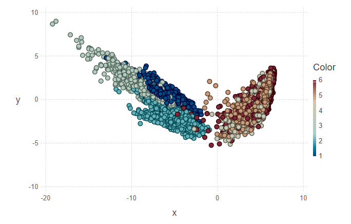
In the first picture, a training sample is laid out and several objects from the test sample that will need to be assigned to their class. Accordingly, the second figure shows that these objects were marked up.

println(z[1][1:10], z[2][1:10])
> [5, 5, 5, 5, 5, 5, 5, 5, 5, 4][1.0, 0.888889, 0.888889, 0.888889, 1.0, 1.0, 1.0, 1.0, 0.777778, 0.555556]

Looking at the images, I want to ask the question "why are such clusters ugly?". I will explain. The individual clusters are not very clearly demarcated due to the nature of the data and the use of PCA. For PCA, simple walking and walking upstairs is like one class — movement class. Accordingly, the second class is the rest class (sitting, standing, lying, which are not very distinguishable between them). And so a clear division can be traced into two classes instead of six.

Conclusion

For me, this is just the initial immersion in Julia and the use of this language in machine learning. By the way, in which I am also more amateur than professional. But while I'm interested, I will continue to study this matter deeper. Many foreign sources place bets on Julia. Well, wait and see.

PS: If it is interesting, I can in the following posts tell about the features of the syntax, about the IDE, with the installation of which I had problems.