HashLife on the knee
After fussing with the three-dimensional game “Life”, I remembered that for an ordinary, convoy version of this game, there is an algorithm called “Hashlife” . It was described in several phrases on Wikipedia, and the picture there with a comment (“configuration through 6 octillion generations”) was enough for me to stay away from this idea: how much resources does this algorithm need? Should I take it at all?
The general idea of the algorithm is this.
Suppose that we have a square of a field of size N * N (N> = 4 is a power of two). Then we can uniquely determine the state of its central region of size (N / 2) * (N / 2) in terms of T = N / 4 steps. If we remember the state of the original square and the result of its evolution in the dictionary, then the next time we meet such a square, we can immediately determine what will become of it.
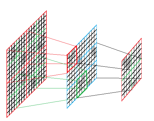
Suppose that for N * N squares we can count the evolution on N / 4 steps. Suppose we have a square 2N * 2N. To calculate its development on N / 2 steps, we can do the following.
Divide the square into 16 squares with side N / 2. We make up 9 squares with side N, for each of them we find the result of evolution by N / 4 steps. Get 9 squares with side N / 2. In turn, we will already make 4 squares of them with side N, and for each of them we will find the result of evolution by N / 4 steps. The resulting 4 squares with side N / 2 will be combined into a square with side N - it will be the answer.
To implement the algorithm, we need to be able to:
If you look for the result of evolution at the time of building the square, then it is enough to have a structure with 5 fields:
Then the algorithm for combining four squares into one can be written as follows:
Actually, that's all. Little things left:
Stop recursion. To do this, all 4 * 4 squares and the results of their evolution by 1 step are entered in the dictionary (in fact, only in this place the program requires knowledge of the rules of the game). For 2 * 2 squares, evolution by half a step is not calculated, they are marked in some special way.
Double the number of evolutionary steps. In terms of the algorithm, this is the same as doubling the size of the square containing the original field. If we want to leave the square in the center, adding zeros to it, we can do this:
Here Zero is a special square, all parts and the result of which are equal to himself.
Or you can simply alternate actions x = Unite (x, Zero, Zero, Zero) and x = Unite (Zero, Zero, Zero, x). The original square will be somewhere in the center.
Implement a dictionary. Here I did not find a beautiful solution: I need to search for the object by key, which is 80% of this object (and not only the remaining 20%, but also the object itself must be searched). Having tinkered with different types of collections, I waved my hand and acted in Fortran: described five integer arrays (LT, RT, LB, RB, Res) and said that the square is determined by an integer –index in these arrays. Indexes from 0 to 15 are reserved for 2 * 2 squares. The sixth array, twice the length, is used for hashing.
You also need to set the field and read the result - but this is a matter of technology. Although you have to be careful with reading: if you execute Expand more than 63 times, the length of the side of the field will cease to fit into 64 bits.
I tested the algorithm on such constructions:
"Garbage Disposer".
It moves at a speed of c / 2, leaves a lot of debris behind it and releases a couple of gliders every 240 steps. A trillion generations (more precisely, 2 ^ 40) were calculated in 0.73 seconds. About 120,000 squares (1,500 for each doubling of time) fell into the dictionary, the number of living cells on the field is 600 billion.
A fragment of the obtained field looks like this:
(2001x2001, 82 KB)
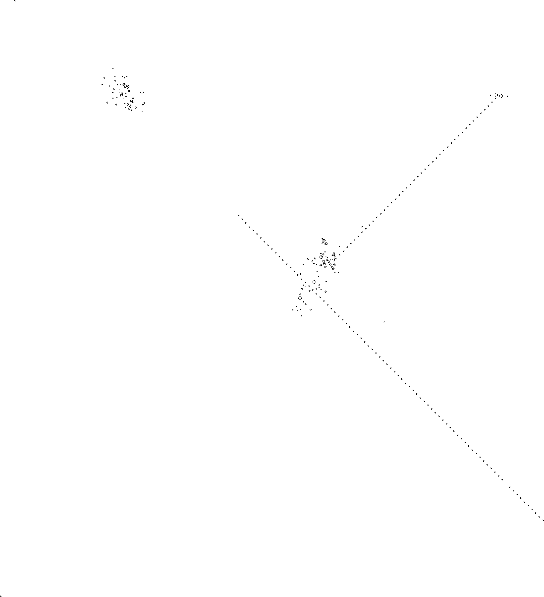
“Battle of glider guns”
Two glider guns are located at a distance of 800 cells from each other, the streams released by them collide:
(T = 2048, 804x504, 11 KB)
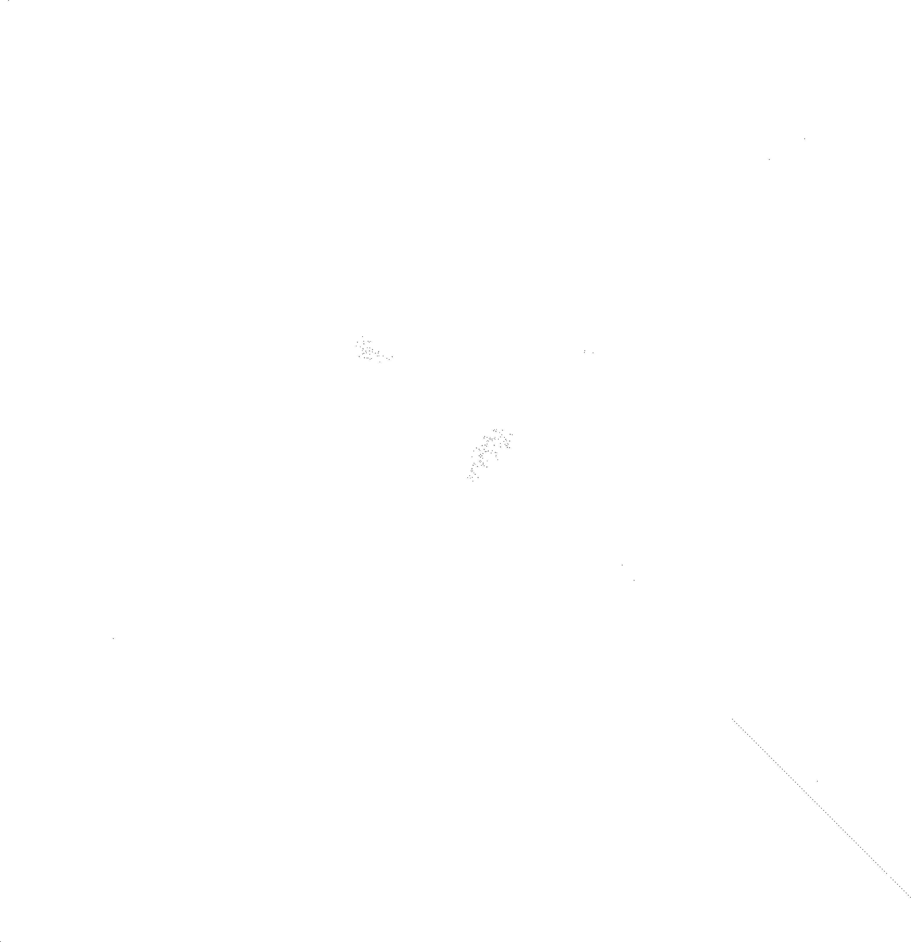
Shortly after the collision, gliders fly out of the pile of debris, which destroy one gun first:
(T = 4096, 1098x1024, 30 Kb)
And then the second one (after which the development quickly ends):
(T = 8192, 3146x3252, 190 Kb)
Counting time - 0.84 seconds, the number of elements in the dictionary - about 270,000.
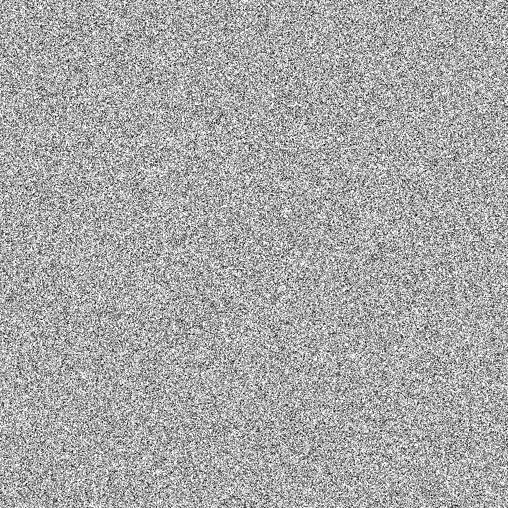
"Random filling" The
field 1024 * 1024 is randomly filled with cells with a density of 1/3. For the algorithm, this is the most difficult case: the configuration stabilizes slowly, and the squares do not begin to repeat immediately.
Here is an example of the development of one of the configurations:
(T = 0, 1024x1024, 300 Kb)
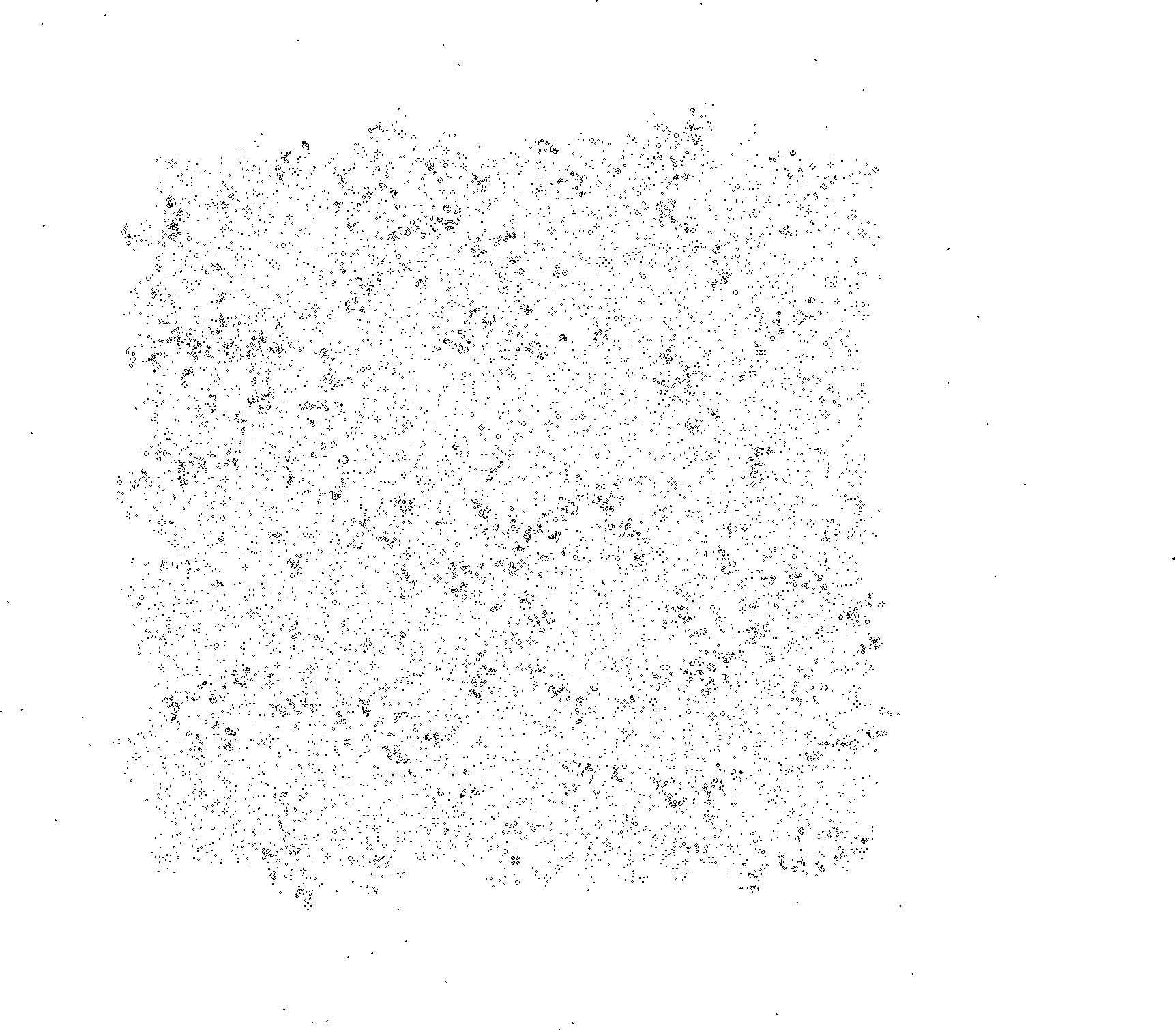
(T = 1024, 1724x1509, 147 Kb)
(T = 2048, 2492x2021, 177 Kb)
(T = 4096, 4028x3045, 300 Kb)
(T = 8192, 7100x5093, 711 Kb)
Counting time - 14 seconds, the number of elements in the dictionary - about 15 million, about 35,000 points remain on the field.
What is unusual in this algorithm? I would note the following:
The general idea of the algorithm is this.
Suppose that we have a square of a field of size N * N (N> = 4 is a power of two). Then we can uniquely determine the state of its central region of size (N / 2) * (N / 2) in terms of T = N / 4 steps. If we remember the state of the original square and the result of its evolution in the dictionary, then the next time we meet such a square, we can immediately determine what will become of it.
Suppose that for N * N squares we can count the evolution on N / 4 steps. Suppose we have a square 2N * 2N. To calculate its development on N / 2 steps, we can do the following.
Divide the square into 16 squares with side N / 2. We make up 9 squares with side N, for each of them we find the result of evolution by N / 4 steps. Get 9 squares with side N / 2. In turn, we will already make 4 squares of them with side N, and for each of them we will find the result of evolution by N / 4 steps. The resulting 4 squares with side N / 2 will be combined into a square with side N - it will be the answer.
To implement the algorithm, we need to be able to:
- Break the square into four squares;
- Find the result of the evolution of the square;
- Find the square consisting of them from the four squares.
If you look for the result of evolution at the time of building the square, then it is enough to have a structure with 5 fields:
class Square {
	internal Square LB, RB, LT, RT, Res;
}
Then the algorithm for combining four squares into one can be written as follows:
Square Unite (Square a0, Square a1, Square a2, Square a3) {
	Square res = FindInDictionary (a0, a1, a2, a3);
	if (res! = null) return res;
// layer at T = N / 4
	Square b1 = Unite (a0.RB, a1.LB, a0.RT, a1.LT) .Res;
	Square b3 = Unite (a0.LT, a0.RT, a2.LB, a2.RB) .Res;
	Square b4 = Unite (a0.RT, a1.LT, a2.RB, a3.LB) .Res;
	Square b5 = Unite (a1.LT, a1.RT, a3.LB, a3.RB) .Res;
	Square b7 = Unite (a2.RB, a3.LB, a2.RT, a3.LT) .Res;
// layer at T = N / 2
	Square c0 = Unite (a0.Res, b1, b3, b4) .Res;
	Square c1 = Unite (b1, a1.Res, b4, b5) .Res;
	Square c2 = Unite (b3, b4, a2.Res, b7) .Res;
	Square c3 = Unite (b4, b5, b7, a3.Res) .Res;
	return AddToDictionary (new Square () {LB = a0, RB = a1, LT = a1, RT = a3, Res = Unite (c0, c1, c2, c3)});
}
Actually, that's all. Little things left:
Stop recursion. To do this, all 4 * 4 squares and the results of their evolution by 1 step are entered in the dictionary (in fact, only in this place the program requires knowledge of the rules of the game). For 2 * 2 squares, evolution by half a step is not calculated, they are marked in some special way.
Double the number of evolutionary steps. In terms of the algorithm, this is the same as doubling the size of the square containing the original field. If we want to leave the square in the center, adding zeros to it, we can do this:
Square Expand (Square x) {
	Square c0 = Unite (Zero, Zero, Zero, x.LB);
	Square c1 = Unite (Zero, Zero, x.RB, Zero);
	Square c2 = Unite (Zero, x.LT, Zero, Zero);
	Square c3 = Unite (x.RT, Zero, Zero, Zero);
	return Unite (c0, c1, c2, c3);
}
Here Zero is a special square, all parts and the result of which are equal to himself.
Or you can simply alternate actions x = Unite (x, Zero, Zero, Zero) and x = Unite (Zero, Zero, Zero, x). The original square will be somewhere in the center.
Implement a dictionary. Here I did not find a beautiful solution: I need to search for the object by key, which is 80% of this object (and not only the remaining 20%, but also the object itself must be searched). Having tinkered with different types of collections, I waved my hand and acted in Fortran: described five integer arrays (LT, RT, LB, RB, Res) and said that the square is determined by an integer –index in these arrays. Indexes from 0 to 15 are reserved for 2 * 2 squares. The sixth array, twice the length, is used for hashing.
You also need to set the field and read the result - but this is a matter of technology. Although you have to be careful with reading: if you execute Expand more than 63 times, the length of the side of the field will cease to fit into 64 bits.
I tested the algorithm on such constructions:
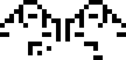
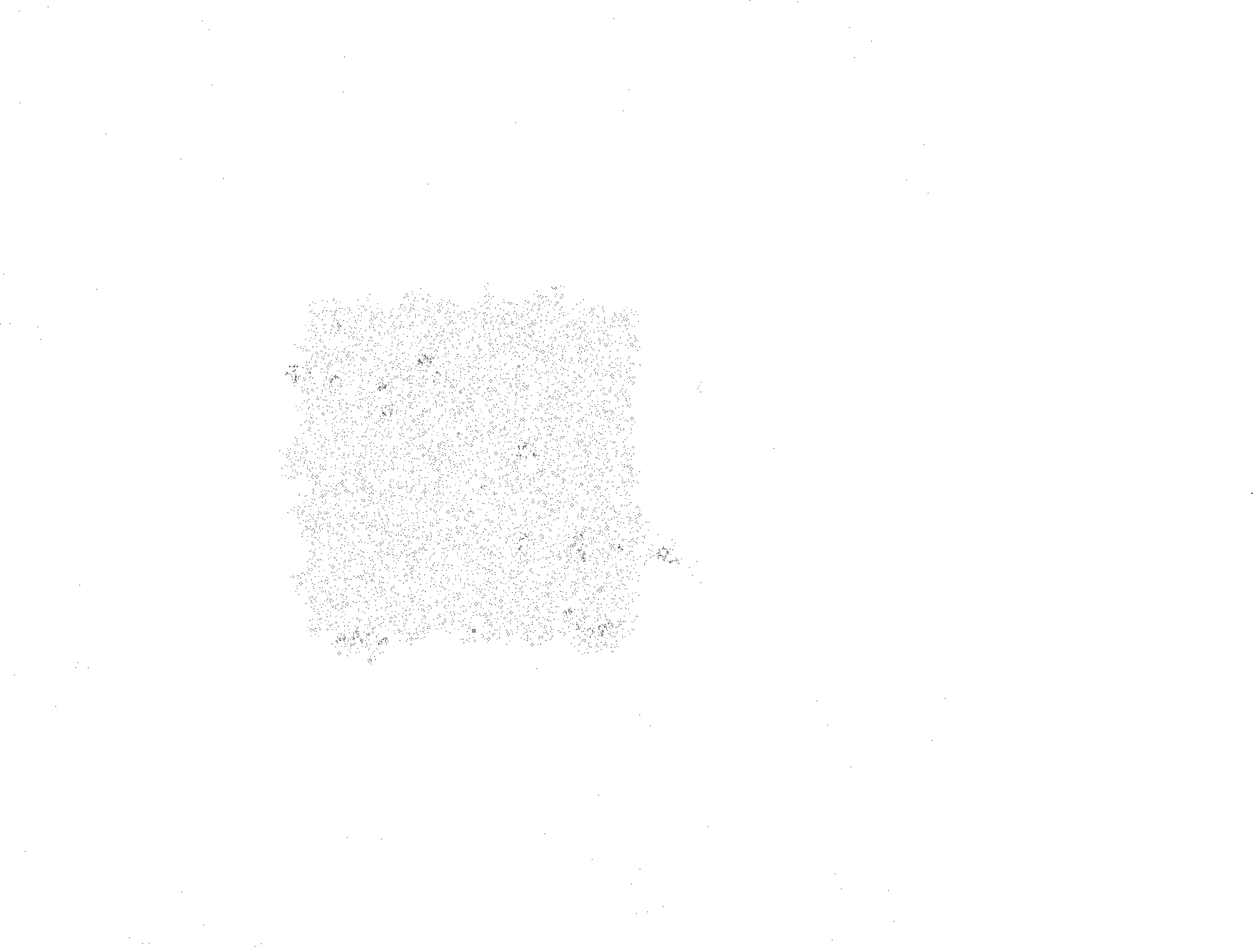
"Garbage Disposer".
It moves at a speed of c / 2, leaves a lot of debris behind it and releases a couple of gliders every 240 steps. A trillion generations (more precisely, 2 ^ 40) were calculated in 0.73 seconds. About 120,000 squares (1,500 for each doubling of time) fell into the dictionary, the number of living cells on the field is 600 billion.
A fragment of the obtained field looks like this:
(2001x2001, 82 KB)
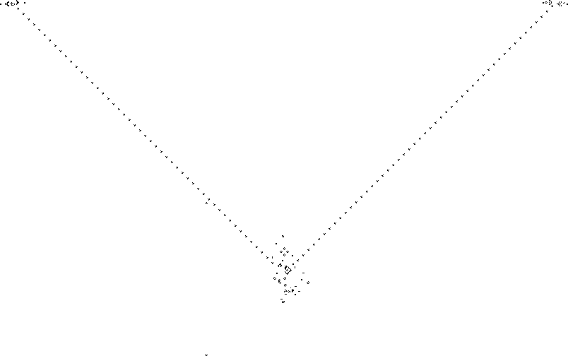
“Battle of glider guns”
Two glider guns are located at a distance of 800 cells from each other, the streams released by them collide:
(T = 2048, 804x504, 11 KB)
Shortly after the collision, gliders fly out of the pile of debris, which destroy one gun first:
(T = 4096, 1098x1024, 30 Kb)
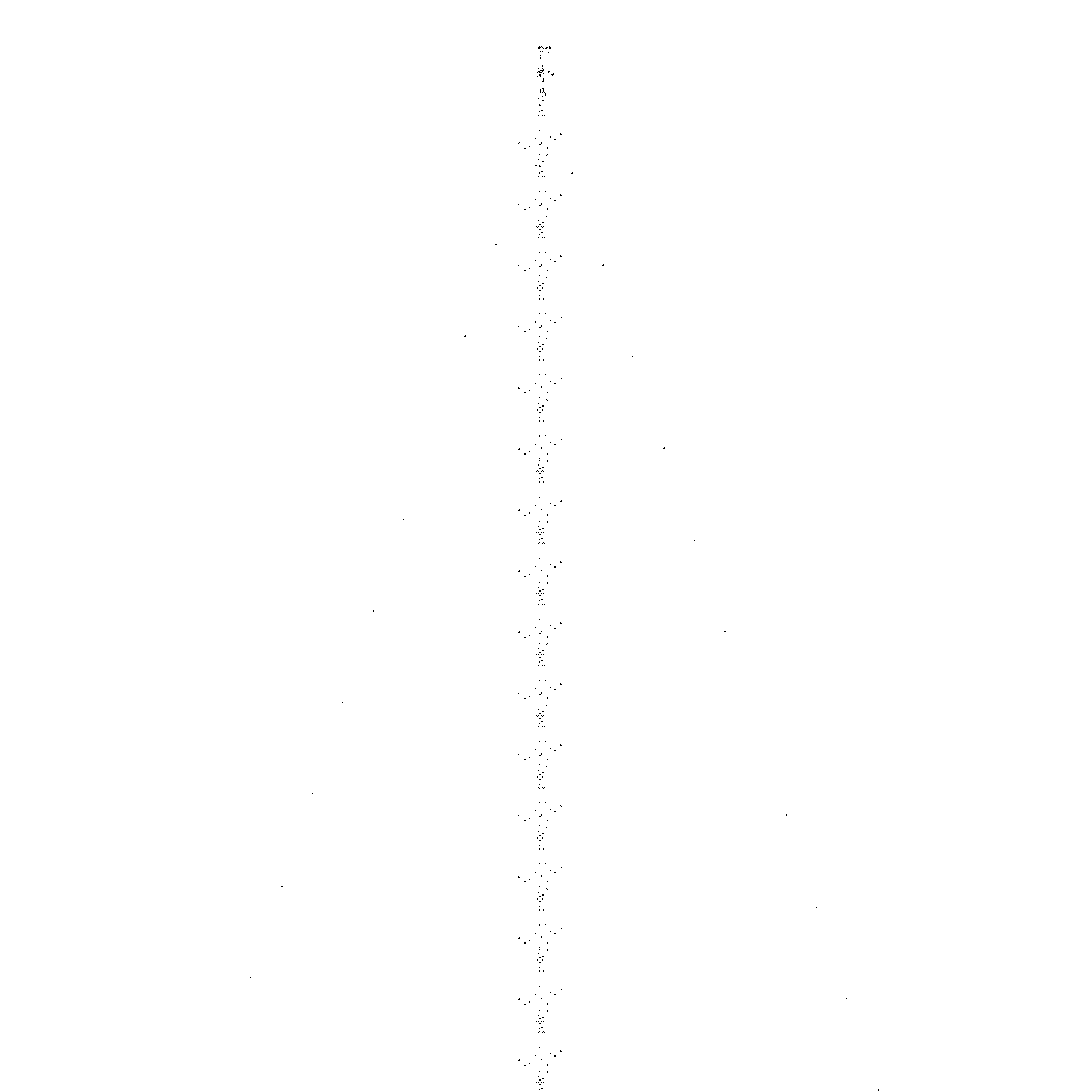
And then the second one (after which the development quickly ends):
(T = 8192, 3146x3252, 190 Kb)
Counting time - 0.84 seconds, the number of elements in the dictionary - about 270,000.
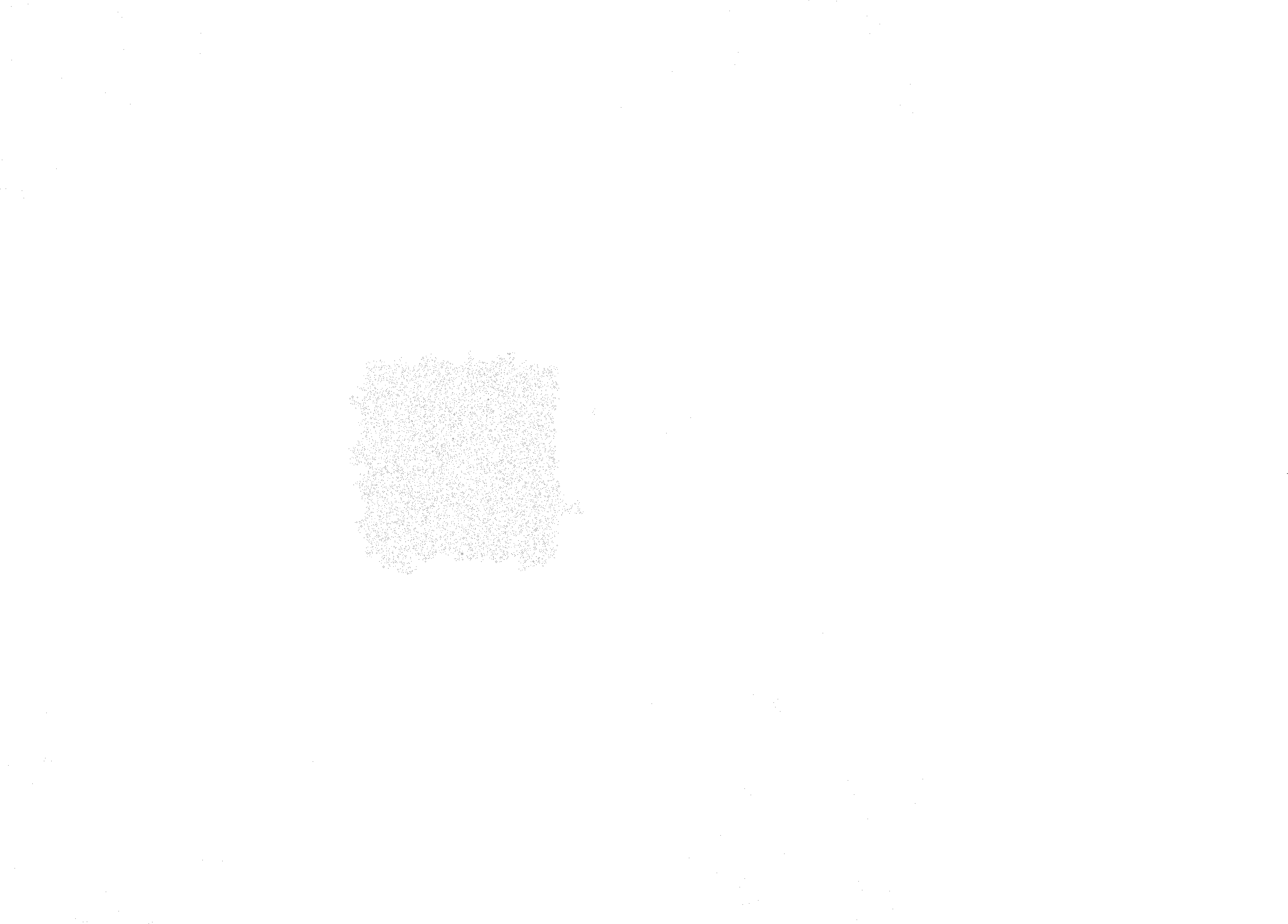
"Random filling" The
field 1024 * 1024 is randomly filled with cells with a density of 1/3. For the algorithm, this is the most difficult case: the configuration stabilizes slowly, and the squares do not begin to repeat immediately.
Here is an example of the development of one of the configurations:
(T = 0, 1024x1024, 300 Kb)
(T = 1024, 1724x1509, 147 Kb)
(T = 2048, 2492x2021, 177 Kb)
(T = 4096, 4028x3045, 300 Kb)
(T = 8192, 7100x5093, 711 Kb)
Counting time - 14 seconds, the number of elements in the dictionary - about 15 million, about 35,000 points remain on the field.
What is unusual in this algorithm? I would note the following:
- Almost without effort, we got a program that can separate empty areas from active ones, track active areas and work out their interaction. If we wrote such an analysis directly, through many dynamic two-dimensional arrays, the program would be much more complicated.
- The algorithm not only calculates the state of the field through T steps - it remembers the entire development. From the result of his work, one can easily extract the state through any interval T_k = 2 ^ k (how to obtain the state of the field after a time that is not a power of two is a separate question). At the same time, the whole evolution turns out to be well-packed - again, without special efforts: 2 ^ 40 generations of the "garbage truck" fit into 3 MB.
- Despite the fact that the dictionary is built according to the initial configuration, its contents do not depend on this configuration. After we have finished some calculation, we can use the same dictionary for the new configuration, and with luck, save a lot of time (though I did not try).
- Formally, the configurations on the plane are presented in the form of 4-trees. But to analyze the interaction between the extreme points of neighboring branches, we do not carry out an explicit descent to these points, but go down only 1-2 steps, after which we look for / build a tree suitable for solving our problem. However, there is nothing unusual here - just that we don’t lose time due to the construction of new nodes, but rather, on the contrary.
- In the algorithm, neither the actual size of the "atomic" cells nor the number of their states is used anywhere. The lowest level to which recursion can go is cells with 16 states, which we perceive as 2 * 2 squares. Space-time at this level (for the algorithm) looks like a face-centered lattice (a three-dimensional chessboard, from which only black cells were taken). The number 16 we invented ourselves based on the rules of Conway. In the algorithm, it could be anything, the main code does not depend on it