One Billion Queens Problem Solution or, “Investigation of the laws in the list of solutions of the n-Queens distribution problem”
Summary
A description is given of the laws that have been established in a sequential list of all solutions to the problem of the distribution of n-Fernets. Determined that:
- The share of complete solutions in the general list of all solutions decreases with increasing value of n.
- Complete solutions are distributed in a sequential list of all solutions in such a way that complete solutions are most likely to occur, located in a list close to each other.
- There is symmetry in order of the location of complete solutions in the general list of all solutions. If the solution in the i-th position from the beginning of the list is complete, then the symmetric solution from the end of the list, located in the n-i + 1 position, is also complete (the rule of symmetry of the solutions).
- Any pairs of solutions, both short and full, located symmetrically in the list of all solutions are complementary - the sum of the indices of the positions of the corresponding lines is constant and equal to n + 1 (the rule of complementarity of the solutions). This suggests that only the first half of the list of all complete solutions is “unique”; any complete solution from the second half of the list can be obtained on the basis of the complementarity rule. The consequence of this rule is the fact that for any value of n, the number of complete solutions will always be an even number.
- The activity of the cells of the rows of the solution matrix is symmetric about the horizontal axis passing through the middle of this matrix. This means that the activity of the cells of the i-th row always coincides with the activity of the cells of the row n-i + 1. By activity is meant the frequency with which the cell index occurs in the corresponding row of the complete solution list. Similarly, the activity of the cells of the columns of the matrix of the solution is symmetrical about the vertical axis dividing the matrix into two equal parts
- Regardless of n, in the sequential search for all solutions, the first complete solution appears only after some sequence of short solutions. The size of the initial sequence of short solutions increases with increasing n. The length of the list of short solutions before the appearance of the first complete solution for even values of n is much longer than for the nearest odd values.
- The row in the decision matrix, on which the difficulties in moving forward, begins, and the first short decision is formed, divides the matrix according to the golden section rule. For small values of n, such a conclusion is approximate; however, with increasing value of n, the accuracy of such a conclusion asymptotically increases to the level of the standard rule.
This publication presents the main results from the article [1] , which was published in the journal "Modeling of Artificial Intelligence, 2018, 5 (1)". On Habré there were works related to the n-Queens problem: [2] , [3] ,
The problem of the distribution of n queens on a nxn chessboard has a long history. It was originally formulated in 1848 by M. Bezzel [4] as an intellectual challenge for an ordinary chessboard. Over time, the formulation of the problem was expanded by F.Nauck [5], and the size of the chessboard could take an arbitrary value.
Introduction
The formulation of the problem is quite simple: you need to distribute n queens on a nxn size chessboard so that each row, each column, and also the left and right diagonals passing through the cell where the queen is located, does not have more than one queen. This task is easy to understand or explain to someone, but it is rather difficult to solve it. The fact is that there are no rules on the basis of which queens can be placed on each line so as to get a solution. The solution can be obtained only on the basis of enumeration of various options for the location of queens in those or other lines. However, the complexity of this solution consists in the fact that the number of all variants of the queens position increases exponentially with increasing n. In addition, the execution of any step forward, for the location of the queen in the free position of a certain string,
There are a large number of publications related to various aspects of solving the problem of n-Queens. They can be attributed to several areas of research: the search for all complete solutions for a given value of the size of a chessboard (n), the development of a fast algorithm to find one solution for different values of n, the solution of the complete set problem to a complete solution, for an arbitrary composition of k queens, questions computational complexity of algorithmic calculations, as well as various modifications of the original formulation of the problem. To get acquainted with these areas, I would recommend interesting publications by B. Jordan, S. Brett [6] and IP Gent, C. Jefferson, P. Nighting [7], which provides a rather detailed overview of various research directions. Of particular note is the online publication [8]supported by Walter Costers, which was prepared by a team from Universiteit Leiden and contains links to 342 publications related to the n-queens problem (as of December 2018).
Although the problem of n-Queens remains active for more than 150 years, and during this time a huge number of publications have appeared, I could not find a job that would be relevant to finding patterns in the results of solving this problem. Most of the projects related to the search for all solutions, most likely did not save the solutions found and did not look at what was “inside there”. There, in the formulation of the problem, there were other dominant goals, and our esteemed colleagues achieved them. However, remotely, it seemed to me that the situation is similar to when a person cooks eggs for breakfast, but does not eat them, but throws them out, leaving only the number of boiled eggs in memory. I have always been convinced that if the data is not random, then there must be a certain regularity in them, even if we cannot find this regularity.
Along with the desire to present useful information for reflection to the members of the Habra community, I would like talented programmers, of whom the majority on Habré, would pay more attention to such a development direction as computer modeling (Computational Simulation). As a research method, such “Algorithmic mathematics” is used on the “leading edge” of many areas: Artificial Intelligence, Software Science, Data Science, ... and I am sure that very complex and important problems for practical application will be solved on the basis of algorithmic mathematics and in no way otherwise.
Definitions
Hereinafter, the size of the chessboard will be denoted by the symbol n. We call a solution complete if all n queens are consistently placed on the chessboard. All other solutions, when the number of correctly placed queens is less than n - we will call short solutions. By the length of the solution, we mean the number (k) of correctly placed queens. The number of all solutions, for a given value of n, will be denoted by the symbol m. As an analogue of a “chessboard” of size nx n., We will consider a “solution matrix” of size nx n.
Start
In order to conduct research, an algorithm was developed to search for all solutions for an arbitrary value n. We did not use standard recursion or the usual nested loop system. For large values of n, such an approach would be quite problematic. The algorithm was built on the basis of a set of interacting events, in each of which, a certain system of actions, interconnected, takes place. This makes it possible to simply implement the mechanism for changing the state space when selecting the next node in the branch of the task solution (Forward tracking), or clearing traces of previously performed actions, when going back one or more steps (Back tracking). The algorithm has no special requirements for the amount of memory or processor speed.
Based on this algorithm, all successive solutions (both short and full) were found for different values of the solution matrix n = (7, ..., 16). Since the size of the list of complete solutions is the named sequence of The On-Line Encyclopedya of Integer Sequences (sequence A000170 [9]) and is indicated in many publications, it seems to me interesting to give the size of the list of all solutions (short + full) for the n values we considered: 7 (194), 8 (736), 9 (2 936), 10 (12 774), 11 (61 076), 12 (314 730), 13 (1 716 652), 14 (10 030 692), 15 ( 62,518,772),16 (415 515 376).
Further, using the solutions found, we will present the formulations of some problems, methods for solving them, and a description of the results obtained.
1. On the state space in which the search for solutions
The enumeration of various variants of the arrangement of queens in one or another row of the matrix of the size n solution leads to the formation of the state space. If there were no restrictions on the location of queens in certain cells of the matrix, then the size of the state space would be equal to n n. If we take into account only the rule prohibiting the location of more than one queen in each row and each column, then we get a subset of the state space, the size of which will be equal to n! This subset of the state space corresponds to the problem of the distribution of n by the rook. If, along with this, we also take into account the rule prohibiting the location of more than one queen on the left and right diagonals passing through the cell where the queen is located, then we will get some search space, the size of which will be less than n! .. Let's call this subset of the state space - productive search space, based on the fact that only in this subspace are all possible solutions. Any completed branches in the productive search space are solutions with a number of correctly placed queens.
Figure 1 shows the graphs of the natural logarithm of three indicators: a) the factorial values (n!) Of the size of the solution matrix; b) the number of all solutions (both short and full); c) the number of complete solutions - depending on the value of the size of the matrix of the solution (n). As expected, all curves exhibit an exponential growth with increasing value of n. The growth rates of the number of all solutions and the number of complete solutions differ, although this is not so noticeable on the graph, due to the small size of the sample of values of n. For example, with n = 13, the difference between the logarithms of these indicators is equal to 3.148, and with n = 16, this difference increases by an amount of 0.190 and is 3.338. Obviously, with a further increase in the value of n, this discrepancy will be more significant.

Fig.1. The dependence of the logarithm of the size of the state space on the value of n
2. How does the share of complete solutions in the general list of all decisions?
It is obvious that if the growth rate of the number of complete solutions lags behind the growth rate of the number of all solutions, then the probability of finding a complete solution in the general list of all solutions will decrease with increasing n. Figure 2 shows a plot of the share of complete solutions in the general list of all solutions of the value of n. It can be seen that with an increase in the size of the solution matrix, the share of all complete solutions in the general list decreases. For the initial values of n = (7, ..., 14), this value decreases 5.66 times from the value of 0.2062 to 0.0364, and then the gradual, asymptotic decrease in this value continues. Here a formal contradiction arises between two statements: on the one hand, the number of complete solutions grows exponentially with increasing value of n, on the other hand, the probability of obtaining a complete solution in a sequential list of all decisions is constantly decreasing. This seeming paradox is explained very simply, the size of the productive space and the associated list size of all solutions grow faster with increasing n than the number of complete solutions. This is like trying to find a needle in a haystack - the amount of hay “with an increase in the value of n” grows faster than the number of needles that were lost there. Therefore, we can assume that if for n = 27, the number of complete solutions is approximately 2.346 * 10 This is like trying to find a needle in a haystack - the amount of hay “with an increase in the value of n” grows faster than the number of needles that were lost there. Therefore, we can assume that if for n = 27, the number of complete solutions is approximately 2.346 * 10 This is like trying to find a needle in a haystack - the amount of hay “with an increase in the value of n” grows faster than the number of needles that were lost there. Therefore, we can assume that if for n = 27, the number of complete solutions is approximately 2.346 * 1017 , then the corresponding value of the number of all solutions will most likely be 3-4 orders of magnitude greater than ~ 10 20
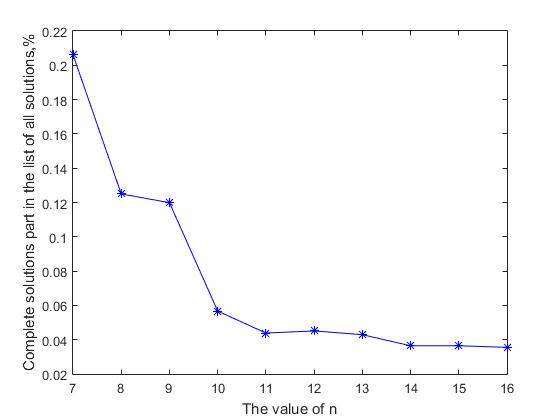
Fig.2 Reduction of the share of complete solutions in the general list of all solutions with an increase in the value of n
3. What is the frequency of decisions of various lengths in the list of all decisions?
As mentioned earlier, all completed branches in the productive search space are solutions with a different number of correctly placed queens.
We are interested in the frequency with which solutions of various lengths are encountered in the general list of all solutions.
Table 1 for the values of n = (7, ..., 12) presents the corresponding values of the relative frequencies for solutions having different lengths. The corresponding visual presentation of this data is shown in Figure 3.
Analysis of the table leads to the following conclusions:
a) for each matrix of size n, there is a certain length of the solution that has a maximum frequency (bold).
| n \ k | four | five | 6 | 7 | eight | 9 | ten | eleven | 12 |
|---|---|---|---|---|---|---|---|---|---|
| 7 | 10.31 | 31.23 | 27.84 | 20.62 | |||||
| eight | 2.45 | 20.38 | 34.78 | 29.89 | 12.50 | ||||
| 9 | 0.34 | 5.79 | 21.73 | 35.83 | 34.32 | 11.99 | |||
| ten | 0.05 | 1.35 | 8.41 | 25.62 | 32.94 | 25.96 | 5.67 | ||
| eleven | 0.15 | 2.12 | 11.80 | 26.71 | 34.47 | 20.36 | 4.39 | ||
| 12 | 0.01 | 0.29 | 3.28 | 13.56 | 29.88 | 31.29 | 17.18 | 4.51 |
b) as the value of n increases, the number of solutions with different lengths increases. Accordingly, this reduces the relative frequency of all decisions.
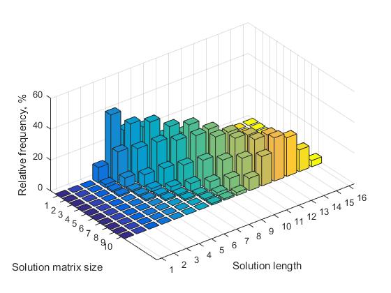
Fig.3. The frequency of solutions of different lengths depending on the size of the solution matrix, n = 7, ..., 16
c) for each matrix of size n, there is a certain minimum size of the length of the solution, below which short solutions do not occur. With increasing value of n, the value of this threshold increases. For example, for n = 8, the threshold value is 4, respectively, with n = 16, the threshold value is 7.
4. What is the relative location of complete solutions in a sequential list of all solutions?
In the formulation of the problem “on the distribution of n queens,” there are no reasons that would give grounds for making any assumption about the sequence of complete solutions in the general list of all solutions. We wondered whether the complete solutions were evenly distributed in the general list, randomly, or it had some peculiarities. To find out, an analysis was made of the distances between the nearest complete solutions in a sequential list of all solutions. As can be seen from Figure 4, where for n = 12, there is a graph of changes in the corresponding frequencies,
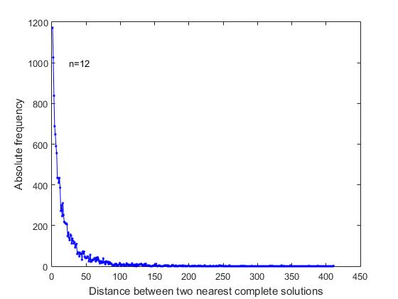
Fig.4. Frequency versus distance between the nearest complete solutions in a sequential list of all complete solutions (n = 12)
with the greatest frequency there are complete solutions that immediately follow each other in the general sequential list of all decisions. These are the cases of the formation of the search branch, when the relationship of free positions in the last lines, allow you to form two or more consecutive full solutions. Further, those full solutions have the maximum frequency, between which there are: one short solution, two short solutions, etc.
5. Is there a pattern in the location of complete solutions in the general list of all solutions?
To answer this question, we analyzed consecutive lists of all solutions for values n = (7, ..., 16). To clearly demonstrate the results obtained, in Figure 5, for the value n = 8, a graph is presented, where the length of each solution is sequentially indicated in the list of all 736 solutions. Here, only 92 solutions are complete, and they are highlighted in red, the remaining 644 solutions are short, and highlighted in blue. It can be seen that the complete solutions are not distributed evenly in the list of all solutions. There are areas where complete solutions are more common, and there are places where complete solutions are rarely found or not found at all.

Fig.5. The length of each decision in a sequential list of all decisions, for a matrix of size 8 x 8 (red - full solutions, blue - short solutions). The total number of all solutions is 736
However, another is important here. If you look closely at the picture, which resembles a blue-red barcode, then you can see one very important feature, all red lines are symmetrical about a certain, conditional vertical line passing through the middle of the list of solutions. In fact, as the verification shows, if at the i-th step from the beginning of the general list there is a complete solution, then, accordingly, the complete solution will necessarily be detected at step m-i + 1. For example, for n = 8, if the first complete solution in the sequential search for all solutions appears at the 43rd step, then accordingly, the last complete solution in the list will be detected at step 736- 43 + 1 = 694. If the 17th solution for a 10x10 matrix appears in the list at the 368th step, then the full solution symmetrical to it will appear in the list of all solutions at step 12774-17 + 1 = 12407. This rule holds for a matrix of solutions of any size. Therefore, we can formulate a rule.For any value of n, if in a sequential list of all decisions, in the i-th position from the beginning of the list, the solution is complete, then a symmetric solution from the end of the list that is in the m-i + 1 position will also be complete (the rule of symmetry of the decisions). Here m, as mentioned above, means the number of all solutions. The consequence of this rule is the fact that for any value of n, the number of complete solutions will always be an even number . (All sizes of the list of complete solutions found so far are even numbers).
If we compare the indices of any two symmetric solutions, we can find a fundamentally important feature - symmetric pairs of solutions are complementary. The sum of the corresponding values of the indices of the queens of symmetric solutions will be equal to n + 1 . For example, the 17th solution for n = 10 in the list of all solutions is in the 368th step from the beginning of the list and the queen position indices at this step are (1, 5, 7, 10, 4, 2, 9, 3, 6, eight).
The corresponding symmetric solution is at step 12407 and has indices of the queen positions (10, 6, 4, 1, 7, 9, 2, 8, 5, 3). If we add the corresponding values of the indices of each pair, we obtain (11, 11, ..., 11). This rule is true for any value of n, and, moreover, both for complete symmetric solutions and for short symmetric solutions. This allows us to formulate the second rule. For a solution matrix of any size n, any pairs of solutions (both short and full), located symmetrically in the sequential list of all decisions, are complementary - the sum of the indexes of the positions of the corresponding rows is constant and equal to n + 1 (the decision complementarity rule). If denoted by Q (i) and Q1 (i) - arrays of indices of complementary solutions, then the rule will be true
<b>`Q ( i ) + Q1 ( i ) = n + 1, i = (1, n) `</b>This generally means that if a complete solution on the i th step, the thus becomes known symmetrical complete solution in step m - i +1. Therefore, when searching for all complete solutions, it suffices to find only the first half of all complete solutions. The second half of the list of complete solutions can be determined from the already obtained solutions, based on the rule of complementarity. The criterion that half of the list of complete solutions has been reached is the fulfillment of the complementarity rule between the previous full solution Q (i-1) and the subsequent Q (i) . ie, it is necessary that the sum of each pair of corresponding values of the indices of two consecutive solutions be equal to n + 1. Since any complete solution from the list of all complete solutions is unique, only those consecutive full solutions will be complementary, which are located on both sides of the border that divides the list in half.
In the future, when searching for all complete solutions for any next value of n, these two rules will reduce the amount of calculations and, accordingly, the counting time by a factor of two.
6. Visualization of the sequence of steps to find the first complete solution.
How does the process of performing the steps forward (Forward tracking) and going back (Back tracking) occur when the decision search branch is formed? In order to answer this question, we, for a 10 x 10 matrix, determined the sequence of the initial 194 transitions between rows before the appearance of the first complete solution. The corresponding graph is shown in Figure 6. The blue lines indicate the movement forward, and the red ones - return back. During these 194 steps, 35 short solutions were created. It can be seen from the figure that most of the transitions (84.5%) occur between the lines (5, 6, 7, 8). It is a kind of “bottleneck” on the way to the “goal”. As follows from the figure, there are only 7 transitions to the 4th row and one transition to the third row. There are also 13 transitions to the 9th row. Three attempts to move to the 10th line were unsuccessful, since there was no free position in these branches of the search on the 10th line. This example clearly demonstrates all the branches of the formation of short

Fig.6 Visualization of Backtracking (red) and Forwardtracking (blue) events for the first 194 search steps (n = 10)
decisions, before receiving the first complete solution. Any algorithm for solving such a problem will be effective if it contains a mechanism that allows you to exclude all (or part of) the branches that lead to short solutions.
7. After how many short solutions does the first complete solution appear?
Considering that complete solutions appear unequally on different parts of the list of all solutions, it seems important to find out how many short solutions appear the first complete solution when searching for all solutions sequentially. For this purpose, for the values n = (7, ..., 35), all short solutions were sequentially computed before the appearance of the first complete solution. As can be seen from Figure 7, which shows a graph of the dependence on n, the natural logarithm of the step number, when the first complete solution appeared, for even values of n, the first complete solution appears much later than for the nearest odd values of n. For example, for an odd value n = 21, the first complete solution appears at step 3138, and for the next, even value n = 22, the first complete solution appears at step 628169. Accordingly, for the following,

Fig.7. The number of short decisions before the appearance of the first complete solution, for different values of n
The number of iteration steps for even n = 22, respectively, 200.2 and 68.6 times more than the nearest odd values. Especially visually on the counting time, this is manifested for n = 34. Here, the first complete solution appears at 826,337,184th step, and for the next odd numbers (33, 35), respectively, at 50,704,900th and 84,888,759th steps. It should also be said about the violation of the monotony of the growth of the number of short solutions before the appearance of the first complete solution, with increasing n. For even values of n, this happens when n = 19, for odd ones, when n = 24 and n = 26.
8. Is the frequency of the cells of each row in the list of all complete solutions the same?
The nxn size decision matrix, which serves as an analogue of a chessboard, is like a scene on which all events occur. Any complete solution formed on this scene consists of cell indices of different rows, since each such cell is a node in the solution search branch. The question that will interest us is this: is the load on each line the same for different cells, when forming a list of all complete solutions? Obviously, the higher the frequency, the higher will be the activity of a given cell in forming a list of complete solutions. To establish this, we define for each line based on the list of all complete solutions, the relative frequency of the various indices. First, we analyze for a solution matrix of size n = 8. Consider successively each row of the storage array of complete solutions and determine the frequency of the various index values. In tables 2, the corresponding values of the absolute frequencies of activity of different cells in each of the eight rows are presented, and in fig. eight
| row \ col | one | 2 | 3 | four | five | 6 | 7 | eight |
|---|---|---|---|---|---|---|---|---|
| one | four | eight | sixteen | 18 | 18 | sixteen | eight | four |
| 2 | eight | sixteen | 14 | eight | eight | 14 | sixteen | eight |
| 3 | sixteen | 14 | four | 12 | 12 | four | 14 | sixteen |
| four | 18 | eight | 12 | eight | eight | 12 | eight | 18 |
| five | 18 | eight | 12 | eight | eight | 12 | eight | 18 |
| 6 | sixteen | 14 | four | 12 | 12 | four | 14 | sixteen |
| 7 | eight | sixteen | 14 | eight | eight | 14 | sixteen | eight |
| eight | four | eight | sixteen | 18 | 18 | sixteen | eight | four |
A group of 4 graphs is presented, where each graph characterizes the change in relative frequencies within a single line. One of the fundamentally important conclusions that can be made on the basis of the analysis of all the data obtained is as follows:
- for a matrix of solutions of arbitrary size n , the activity of the cells of the i -th row coincides with the activity of the cell n-i + 1 , i.e. the activity of the cells of the first row always coincides with the activity of the cells of the last row, respectively, the activity of the cells of the second row coincides with the activity of the cells of the penultimate row, etc.
If n is odd, only the median row of the solution matrix does not have a symmetric pair, for all other cells the above rule is true - Let's call this “the property of the horizontal symmetry of the activity of cells of different rows of the solution matrix” . For this reason, we presented only 4 graphs for a matrix of size n = 8, since the corresponding cell activity graphs for rows (1, 8), (2.7), (3.6) and (4.5) are completely identical.
It should also be noted that the values of frequencies are symmetric about the vertical axis of the dividing matrix into two equal parts (in the case of an even value of n), or passing through the median column (in the case of an odd value of n). Let's call this “the property of the vertical symmetry of the activity of cells of different rows of the solution matrix” .
In addition, as follows from the analysis of table 2, the frequencies in the matrix of the solution are symmetric with respect to the left and right main diagonals.
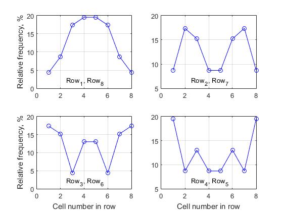
Fig.8. The activity of the cells of the corresponding rows when forming the list of complete solutions, n = 8
I think that the presence of restrictive rules in the formulation of the problem, and the property of non-determinism associated with this, “form” a kind of harmonious relationship between nodes in different lines. Those branches of the search that fit into these rules lead to the formation of a complete solution. The remaining branches of the search, at some step, violate these rules, and as a result, “complete their path” in the form of short decisions. It should be noted here that the cells of the decision matrix have only a local relationship within the projection influence group, there are no prescribed rules on coordinated actions between them. The collective activity of the cells is only a consequence of the impact of the restrictive rules. Therefore, it remains an open rather interesting question of how limiting rules, as non-determinism factors, affect the cells of the decision matrix, which ultimately leads to the formation of a “harmonious” matrix of the activity of the cells - symmetrical about the horizontal and vertical axes, as well as about the left and right diagonals. Is this a characteristic property only of a given task, or does it also exist for other non-deterministic problems?
9. From which line number does the Forward tracking - Back tracking algorithm turn on?
If you follow the work of the algorithm for sequential selection of rows in the decision matrix for the location of the queen, you can see that starting with a certain line, which we call “StopRow”, the process of moving forward is “braked”. In the search branch, such a line is the first where problems arise with the presence of free

Fig. 9-1 Dependence of the ratio of the StopRow index to n on the size of the decision matrix (part-1)
position for the location of the queen. It is from this line that the Back tracking algorithm is turned on for clearing traces of previously performed actions, and going back. This is the line on which the first short decision appears.
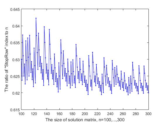
Fig.9-2 Dependence of the ratio of the StopRow index to n on the size of the solution matrix (part-2)
The index of the “StopRow” row, from which the difficulties in moving forward, begins, depends on the size n of the decision matrix. If we consider the ratio of this index, which we denote by StopInd to the size of the matrix of the solution n, then, as can be seen from Figure 9-1, where the calculation results for the initial values n = (7, ..., 99) are presented, this ratio fluctuates more or less side and tends to decrease. With an increase in the value of n = (100, ..., 300), this ratio fluctuates within 0.619 - 0.642 (Fig. 9-2), and with a further increase in n, we get the following results (the values of n are given sequentially, and StopInd and the ratio StopInd / n: 1000 (619, 0.6190), 2000 (1239, 0.6195), 3000 (1856, 0.6187), 4000(2473, 0.6182), 5000 (3091, 0.6182). Surprisingly, it can be argued that the stop line divides the decision matrix according to the golden section rule : namely, the StopInd / n ratio differs from (n-StopInd) / StopInd by a small amount, which tends to zero with increasing n. For example, for n = 5000, the difference between the ratios 3091/5000 and 1909/3091 is 0.006, which is less than 0.1% of the average of these two ratios.
The graph presented in two figures. 9- (1,2) has a non-random form of variability, which resembles the recording on the "musical music band". One can see repeated jumps upwards and a stepped fall downwards with some irregular periodicity. Obviously, there is a certain reason for such a behavior of the curve, and perhaps this will be of interest for the study. For this reason, for the purpose of more detailed visualization, the graph was presented in two figures.
I have considered only a part of the questions that can be formulated on the basis of the results of solving the problem “on the distribution of n-queens”. I hope that the results will make more transparent for understanding the mechanisms of formation of non-deterministic processes and changes in the state space. Perhaps this will serve as a foothold for the formulation of new tasks and the way forward.
Conclusion
- If, looking through the publication, we have reached the conclusion, then naturally the question will arise: “what's the One Billion Queens Problem Solution in the title of the article?” Preparing the publication for Habr, I thought that a person who, for example, possesses a mine where diamonds are mined, should donate at least one diamond to his friends and relatives, otherwise it would be unfair. Therefore, I would like to present a gift to all members of the habr-community: participants, organizers, visitors. As the name suggests, this is a solution to the problem of the distribution of one billion queens on a billion-billion-dollar chessboard.
Of course, this is not a faceted diamond, but for true connoisseurs of intellectual art, it may be more valuable than "some kind of diamond." Moreover, there are many different diamonds around the world, and this solution is so far only in one copy. And sees our Byte-God (*), that I do it sincerely.
The resulting solution is a one-dimensional array consisting of one billion numbers, which is presented in MatLab .mat format and is available at: One Billion Queens Problem Solution on Google Drive
- The first element of this array characterizes the position of the queen in the first line, the second element - the position in second line, etc. This is only one solution from nBillion possible solutions. And the value of nBillion is so large that it can be considered a close relative of infinity. - It seems to me that this solution can be attributed to the category of virtual intellectual values. We can say that "this is something in which something is." They cannot really be touched, so it is perceived in consciousness only at the level of sensations. There, in fact, there is an amazing order and explicit and implicit harmony. This is a purely symbolic gift (in the literal and figurative sense), which is addressed to all members of the community. I think that " you are not like everyone else ."
(I hope that someone will "take the gift home." The file is quite large - 3.7 Gb. This is clean, verified data. The fact that Google Drive will display warnings - treat this with understanding) - Before making this decision, I thought about the individual-collective nature of such a gift. Does it not turn out that the original will be given to one and the rest to the copy? But the solution was simple. The familiar “everyday” concepts of “original” and “copy” in this case lose their meaning. We do not copy, and create another original. And the "originals" for all are the same and equally equivalent.
- I think that in the company of relatives, you will most likely be the only one who received such an “intellectual product” as a gift. It will be fun if you tell your mother-in-law about such a gift: “Imagine a mother’s chessboard measuring 50,000 km per 50,000 km, on which 1 billion queens are distributed in such a way that one does not see one another at rest ...”. Who knows, maybe after that, his son-in-law will appreciate more, since he is being given such a strange gift.
I wish all members of the habr-community health, success and well-being. May the new year bring us all good luck.
(*) - Since I referred to the name of an object, its description should also be given.
Byte-God means a multidimensional entity consisting of zeroes and ones, rational in all senses and infinite in all directions. Any sequence of zeros and ones in this space represents certain knowledge.
Bibliography
[4] Max Bezzel, Proposal of 8-queens problem ", Berliner Schachzeitung, Volume
3 (1848), page 363. (Submitted under the author name \ Schachfreund".)
[5] Franz Nauck, Briefwechseln mit allen fur alle ", Illustrirte Zeitung, Volume
377 Number 15 (1850), page 182.
[6] Bell Jordan; Stevens Brett (2009). "A survey of known results and research areas for n-queens". Discrete Mathematics. 309 (1): 1–31
[7] Gent, Ian P .; Jefferson, Christopher; Nightingale, Peter (August 2017). "Complexity of n-Queens Completion". Journal of Artificial Intelligence Research. AAAI Press. 59: 815–848
[8] W. Kosters and all, n-Queens - 342 references, (November 20, 2018)
[9] NJA Sloane, the On-Line Encyclopedia of Integer Sequences, electronically published. 2016