Introduction to Algorithm A *
- Transfer
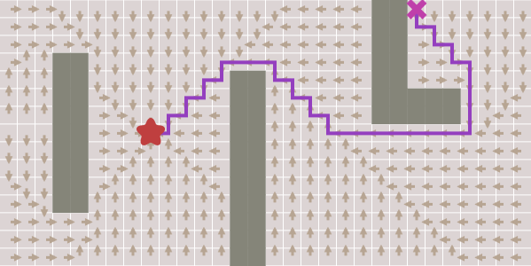
When developing games, we often need to find ways from one point to another. We do not just strive to find the shortest distance, we also need to take into account the duration of the movement. Move the asterisk (start point) and cross (end point) to see the shortest path. [Note per .: in the articles of this author there are always many interactive inserts, I recommend that you go to the original article.]
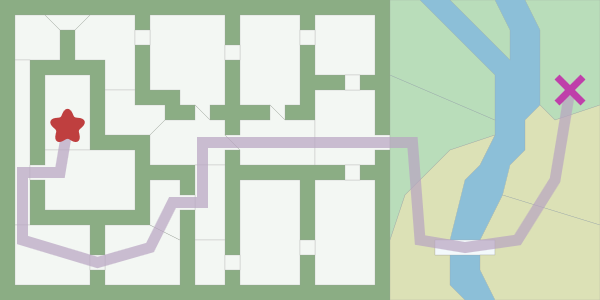
To search for this path, you can use the graph search algorithm, which is applicable if the map is a graph. A * is often used as a graph search algorithm. The breadth -first search is the simplest of the graph search algorithms, so let's start with it and gradually move on to A *.
The first thing you need when learning an algorithm is to understand the data . What is served at the entrance? What do we get on the way out?
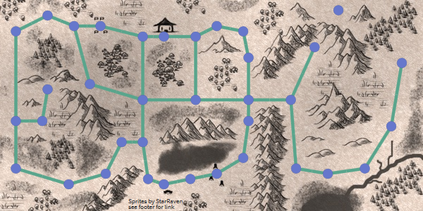
Input : graph search algorithms, including A *, receive a graph as input. A graph is a set of points (“nodes”) and connections (“edges”) between them. Here is the graph I passed to A *:

A * does not see anything else. He sees only the count. He does not know if something is in the room or outside, whether it is a door or a room, how large the area is. He sees only the count! He does not understand any difference between the card on top and this one:
Exit: A * defined path consists of nodes and edges. Ribs are an abstract mathematical concept. A * tells us that we need to move from one point to another, but does not tell how to do it. Remember that he does not know anything about rooms or doors, he sees only the count. You yourself must decide what the edge of the graph will be, returned by A * - moving from tile to tile, moving in a straight line, opening a door, running along a curved path.
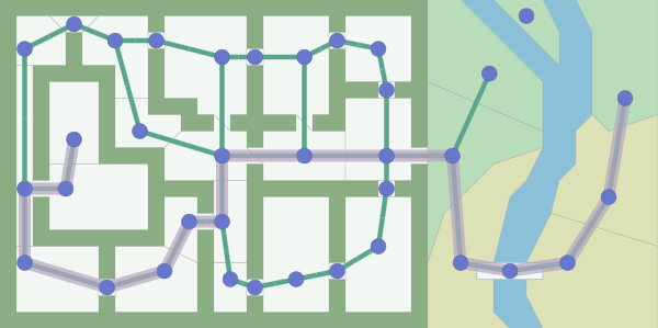
Trade-offs: For each game card, there are many different ways to pass the path search graph to the A * algorithm. The map in the figure above turns the doors into nodes.
But what if we turn the doors into ribs?

And if we use the grid to find the path?
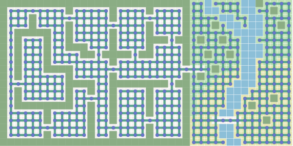
The path search graph does not have to be the same as that used on your game map. In a grid-based map, you can use the path search graph without meshes, and vice versa. A * runs faster with the least number of graph nodes. Grids are often easier to work with, but they produce many nodes. This article discusses the A * algorithm itself, not the graph design. More information about graphs can be found on my other page . For further explanation, I will use grids in the future , because it is easier to visualize concepts .
There are many algorithms that work with graphs. I will consider the following:

A breadth-first search performs research evenly in all directions. This is an incredibly useful algorithm, not only for the usual search for the path, but also for the procedural generation of maps, search for flow paths, distance maps and other types of map analysis.

Dijkstra's algorithm (also called uniform-cost search) allows us to prioritize path research. Instead of exploring all the possible paths evenly, he prefers low-cost paths. We can set reduced costs so that the algorithm moves along roads, increased cost, to avoid forests and enemies, and much more. When the cost of movement can be different, we use it instead of the breadth-first search.

A *Is a modification of Dijkstra's algorithm, optimized for a single endpoint. Dijkstra's algorithm can find paths to all points, A * finds a path to one point. He gives priority to paths that lead closer to the goal.
I will start with the simplest - breadth-first search, and I will add functions, gradually turning it into A *.
The key idea of all these algorithms is that we track the state of the expanding ring, which is called the boundary . In a grid, this process is sometimes called flood fill, but the same technique applies to cards without meshes. Watch the border extension animation:
How to implement this? Repeat these steps until the border is empty:
Let's take a closer look at this. Tiles are numbered in the order they are visited:
The algorithm is described in just ten lines of Python code:
In this cycle, the whole essence of the search algorithms in the graph of this article, including A *, lies. But how do we find the shortest path? The cycle does not actually create paths, it just tells us how to visit all the points on the map. This happened because the breadth-first search can be used for much more than just a path search. In this article I show how it is used in tower defense games, but it can also be used in distance maps, in procedural map generation, and much more. However, here we want to use it to find paths, so let's change the loop so that it tracks where we came from for each visited point and rename it
Now came_from for each point indicates the place from which we came. It is like the bread crumbs from a fairy tale. This is enough for us to recreate the whole path. See how the arrows show the way back to the starting position.
The code to recreate the paths is simple: follow the arrows back from the target to the beginning . A path is a sequence of edges , but sometimes it’s easier to store only nodes:
This is the simplest path finding algorithm. It works not only in grids, as shown above, but also in any graph structure. In a dungeon, points in a graph can be rooms, and edges can be doors between them. In the platformer, the nodes of the graph can be locations, and the edges can be possible actions: move left, right, jump, jump down. In general, you can perceive the graph as states and actions that change the state. I wrote more about the presentation of maps here . In the remainder of this article, I will continue to use examples with meshes, and talk about why you can use a variety of searches in width.
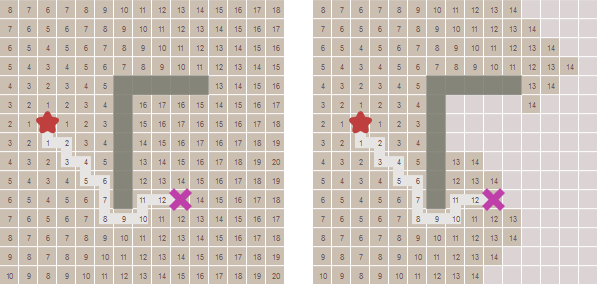
We found paths from one point to all other points. Often we don’t need all the paths, we just need a path between two points. We can stop expanding the border as soon as we find our goal. See how the border ceases to expand after finding the target.
The code is fairly straightforward:
So far we have taken steps with the same value. In some cases, finding paths for different types of traffic has different costs. For example, in Civilization, movement through the plains or desert may cost 1 movement point, and movement through the forest may cost 5 movement points. On the map at the very beginning of the article, passing through water costs 10 times more than moving along the grass. Another example is the diagonal movement in the grid, which costs more than the movement along the axes. We need a path search to take this cost into account. Let's compare the number of steps from the beginning to the distance from the beginning:

For this we need the Dijkstra algorithm(also called uniform cost searches). How does it differ from breadth-first search? We need to track the cost of movement, so add a new variable
Using a priority queue instead of a regular queue changes the way the border expands . Contour lines allow you to see this. Watch the video to watch how the border expands more slowly through the forests, and the shortest path is searched around the central forest, and not through it:
The cost of movement, which differs from 1, allows us to explore more interesting graphs, not just grids. On the map at the beginning of the article, the cost of movement is based on the distance between the rooms. Movement cost can also be used to avoid or prefer areas based on the proximity of enemies or allies. An interesting implementation detail: a regular priority queue supports insert and delete operations, but some versions of Dijkstra's algorithm also use the third operation, which changes the priority of an element already in the priority queue. I do not use this operation, and explain it on the algorithm implementation page .
In the breadth-first search and Dijkstra's algorithm, the border expands in all directions. This is a logical choice if you are looking for a way to all points or to many points. However, usually a search is performed for only one point. Let's make the border expand towards the goal more than in other directions. First, we define a heuristic function that tells us how close we are to the goal:
In Dijkstra’s algorithm, we used the distance from the beginning to order the priority queue . In the greedy search for the first best match for priority order, we use the estimated distance to the target instead . The point closest to the target will be examined first. The code uses a queue with priorities from the breadth-first search, but it is not used
Let's see how it works:
Wow! Amazing, right? But what will happen on a more complex map?
These paths are not shortest. So, this algorithm works faster when there are not very many obstacles, but the paths are not too optimal. Can this be fixed? Of course.
Dijkstra's algorithm is good at finding the shortest path, but he spends time exploring all directions, even unpromising ones. Greedy search explores promising directions, but may not find the shortest path. The A * algorithm uses both the true distance from the start and the estimated distance to the target.
The code is very similar to Dijkstra's algorithm:
Compare the algorithms: Dijkstra's algorithm calculates the distance from the starting point. A greedy search by the first best match estimates the distance to the target point. A * uses the sum of these two distances.
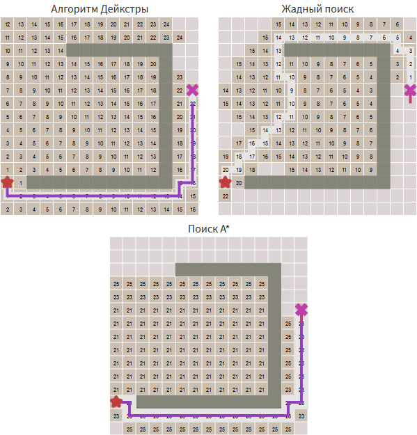
Try to make holes in different places of the wall in the original article. You will find that the greedy search finds the correct answer, A * also finds it, exploring the same area. When a greedy search on the first best finds the wrong answer (a longer path), A * finds the correct one, like Dijkstra’s algorithm, but still investigates less than Dijkstra’s algorithm.
A * takes the best from two algorithms. Since the heuristic does not re-evaluate distances, A * does notuses heuristics to find a suitable answer. He finds the optimal path, like the Dijkstra algorithm. A * uses heuristics to change the order of nodes to increase the likelihood of finding the target node earlier.
And that is all! This is the algorithm A *.
Are you ready to implement it? Try using a ready-made library. If you want to implement it yourself, then I have instructions for step-by-step implementation of graphs, queues and path search algorithms in Python, C ++ and C #.
What algorithm should be used to find paths on the game map?
What about the best ways? The breadth-first search and Dijkstra's algorithm are guaranteed to find the shortest path in the graph. A greedy search will not necessarily find it. A * is guaranteed to find the shortest path if the heuristic is never greater than the true distance. When the heuristic becomes smaller, A * turns into Dijkstra's algorithm. When the heuristic gets larger, A * turns into a greedy search for the best first match.
What about performance? It is best to eliminate unnecessary points in the graph. If you use a grid, then read this.. Reducing graph size helps all graph search algorithms. After that, use the simplest possible algorithm. Simple queues run faster. Greedy searches are usually faster than Dijkstra's algorithm, but do not provide optimal paths. For most path finding tasks, the best choice is A *.
What about using not on maps? I used maps in the article because I think it’s easier to explain the operation of the algorithm on them. However, these graph search algorithms can be used on any graphs, not only on game cards, and I tried to present the algorithm code in a form independent of two-dimensional grids. The cost of movement on maps turns into arbitrary weights of the edges of the graph. Transferring heuristics to arbitrary cards is not so simple; you need to create heuristics for each type of graph. For flat maps, distances are a good choice, so here we used them.
I wrote a lot more about finding paths here. Remember that graph search is only one part of what you need. By itself, A * does not handle such aspects as joint movement, moving obstacles, changing a map, assessing dangerous areas, formations, turning radii, object sizes, animation, smoothing paths and much more.
To search for this path, you can use the graph search algorithm, which is applicable if the map is a graph. A * is often used as a graph search algorithm. The breadth -first search is the simplest of the graph search algorithms, so let's start with it and gradually move on to A *.
Map view
The first thing you need when learning an algorithm is to understand the data . What is served at the entrance? What do we get on the way out?
Input : graph search algorithms, including A *, receive a graph as input. A graph is a set of points (“nodes”) and connections (“edges”) between them. Here is the graph I passed to A *:
A * does not see anything else. He sees only the count. He does not know if something is in the room or outside, whether it is a door or a room, how large the area is. He sees only the count! He does not understand any difference between the card on top and this one:
Exit: A * defined path consists of nodes and edges. Ribs are an abstract mathematical concept. A * tells us that we need to move from one point to another, but does not tell how to do it. Remember that he does not know anything about rooms or doors, he sees only the count. You yourself must decide what the edge of the graph will be, returned by A * - moving from tile to tile, moving in a straight line, opening a door, running along a curved path.
Trade-offs: For each game card, there are many different ways to pass the path search graph to the A * algorithm. The map in the figure above turns the doors into nodes.
But what if we turn the doors into ribs?
And if we use the grid to find the path?
The path search graph does not have to be the same as that used on your game map. In a grid-based map, you can use the path search graph without meshes, and vice versa. A * runs faster with the least number of graph nodes. Grids are often easier to work with, but they produce many nodes. This article discusses the A * algorithm itself, not the graph design. More information about graphs can be found on my other page . For further explanation, I will use grids in the future , because it is easier to visualize concepts .
Algorithms
There are many algorithms that work with graphs. I will consider the following:
A breadth-first search performs research evenly in all directions. This is an incredibly useful algorithm, not only for the usual search for the path, but also for the procedural generation of maps, search for flow paths, distance maps and other types of map analysis.
Dijkstra's algorithm (also called uniform-cost search) allows us to prioritize path research. Instead of exploring all the possible paths evenly, he prefers low-cost paths. We can set reduced costs so that the algorithm moves along roads, increased cost, to avoid forests and enemies, and much more. When the cost of movement can be different, we use it instead of the breadth-first search.
A *Is a modification of Dijkstra's algorithm, optimized for a single endpoint. Dijkstra's algorithm can find paths to all points, A * finds a path to one point. He gives priority to paths that lead closer to the goal.
I will start with the simplest - breadth-first search, and I will add functions, gradually turning it into A *.
Wide search
The key idea of all these algorithms is that we track the state of the expanding ring, which is called the boundary . In a grid, this process is sometimes called flood fill, but the same technique applies to cards without meshes. Watch the border extension animation:
How to implement this? Repeat these steps until the border is empty:
- Select and delete a point from the border .
- We mark the point as visited in order to know that we do not need to process it again.
- Expanding the border, looking at its neighbors . We add all the neighbors that we have not yet seen to the border .
Let's take a closer look at this. Tiles are numbered in the order they are visited:
The algorithm is described in just ten lines of Python code:
frontier = Queue()
frontier.put(start )
visited = {}
visited[start] = True
while not frontier.empty():
   current = frontier.get()
   for next in graph.neighbors(current):
      if next not in visited:
         frontier.put(next)
         visited[next] = True
In this cycle, the whole essence of the search algorithms in the graph of this article, including A *, lies. But how do we find the shortest path? The cycle does not actually create paths, it just tells us how to visit all the points on the map. This happened because the breadth-first search can be used for much more than just a path search. In this article I show how it is used in tower defense games, but it can also be used in distance maps, in procedural map generation, and much more. However, here we want to use it to find paths, so let's change the loop so that it tracks where we came from for each visited point and rename it
visitedto came_from:frontier = Queue()
frontier.put(start )
came_from = {}
came_from[start] = None
while not frontier.empty():
current = frontier.get()
for next in graph.neighbors(current):
if next not in came_from:
frontier.put(next)
came_from[next] = currentNow came_from for each point indicates the place from which we came. It is like the bread crumbs from a fairy tale. This is enough for us to recreate the whole path. See how the arrows show the way back to the starting position.
The code to recreate the paths is simple: follow the arrows back from the target to the beginning . A path is a sequence of edges , but sometimes it’s easier to store only nodes:
current = goal
path = [current]
while current != start:
   current = came_from[current]
   path.append(current)
path.append(start) # optional
path.reverse() # optional
This is the simplest path finding algorithm. It works not only in grids, as shown above, but also in any graph structure. In a dungeon, points in a graph can be rooms, and edges can be doors between them. In the platformer, the nodes of the graph can be locations, and the edges can be possible actions: move left, right, jump, jump down. In general, you can perceive the graph as states and actions that change the state. I wrote more about the presentation of maps here . In the remainder of this article, I will continue to use examples with meshes, and talk about why you can use a variety of searches in width.
Early exit
We found paths from one point to all other points. Often we don’t need all the paths, we just need a path between two points. We can stop expanding the border as soon as we find our goal. See how the border ceases to expand after finding the target.
The code is fairly straightforward:
frontier = Queue()
frontier.put(start )
came_from = {}
came_from[start] = None
while not frontier.empty():
   current = frontier.get()
   if current == goal:
      break
   for next in graph.neighbors(current):
      if next not in came_from:
         frontier.put(next)
         came_from[next] = current
Moving cost
So far we have taken steps with the same value. In some cases, finding paths for different types of traffic has different costs. For example, in Civilization, movement through the plains or desert may cost 1 movement point, and movement through the forest may cost 5 movement points. On the map at the very beginning of the article, passing through water costs 10 times more than moving along the grass. Another example is the diagonal movement in the grid, which costs more than the movement along the axes. We need a path search to take this cost into account. Let's compare the number of steps from the beginning to the distance from the beginning:
For this we need the Dijkstra algorithm(also called uniform cost searches). How does it differ from breadth-first search? We need to track the cost of movement, so add a new variable
cost_so_farto monitor the total cost of movement from the starting point. When evaluating points, we need to consider the cost of movement. Let's turn our queue into a priority queue. Less obvious is that it can happen that one point is visited several times with different costs, so you need to slightly change the logic. Instead of adding a point to the border when we have never visited a point, we add it if the new path to the point is better than the best previous path.frontier = PriorityQueue()
frontier.put(start, 0)
came_from = {}
cost_so_far = {}
came_from[start] = None
cost_so_far[start] = 0
while not frontier.empty():
current = frontier.get()
if current == goal:
break
for next in graph.neighbors(current):
new_cost = cost_so_far[current] + graph.cost(current, next)
if next not in cost_so_far or new_cost < cost_so_far[next]:
cost_so_far[next] = new_cost
priority = new_cost
frontier.put(next, priority)
came_from[next] = currentUsing a priority queue instead of a regular queue changes the way the border expands . Contour lines allow you to see this. Watch the video to watch how the border expands more slowly through the forests, and the shortest path is searched around the central forest, and not through it:
The cost of movement, which differs from 1, allows us to explore more interesting graphs, not just grids. On the map at the beginning of the article, the cost of movement is based on the distance between the rooms. Movement cost can also be used to avoid or prefer areas based on the proximity of enemies or allies. An interesting implementation detail: a regular priority queue supports insert and delete operations, but some versions of Dijkstra's algorithm also use the third operation, which changes the priority of an element already in the priority queue. I do not use this operation, and explain it on the algorithm implementation page .
Heuristic Search
In the breadth-first search and Dijkstra's algorithm, the border expands in all directions. This is a logical choice if you are looking for a way to all points or to many points. However, usually a search is performed for only one point. Let's make the border expand towards the goal more than in other directions. First, we define a heuristic function that tells us how close we are to the goal:
def heuristic(a, b):
   # Manhattan distance on a square grid
   return abs(a.x - b.x) + abs(a.y - b.y)
In Dijkstra’s algorithm, we used the distance from the beginning to order the priority queue . In the greedy search for the first best match for priority order, we use the estimated distance to the target instead . The point closest to the target will be examined first. The code uses a queue with priorities from the breadth-first search, but it is not used
cost_so_farfrom Dijkstra's algorithm:frontier = PriorityQueue()
frontier.put(start, 0)
came_from = {}
came_from[start] = None
while not frontier.empty():
current = frontier.get()
if current == goal:
break
for next in graph.neighbors(current):
if next not in came_from:
priority = heuristic(goal, next)
frontier.put(next, priority)
came_from[next] = currentLet's see how it works:
Wow! Amazing, right? But what will happen on a more complex map?
These paths are not shortest. So, this algorithm works faster when there are not very many obstacles, but the paths are not too optimal. Can this be fixed? Of course.
Algorithm A *
Dijkstra's algorithm is good at finding the shortest path, but he spends time exploring all directions, even unpromising ones. Greedy search explores promising directions, but may not find the shortest path. The A * algorithm uses both the true distance from the start and the estimated distance to the target.
The code is very similar to Dijkstra's algorithm:
frontier = PriorityQueue()
frontier.put(start, 0)
came_from = {}
cost_so_far = {}
came_from[start] = None
cost_so_far[start] = 0
while not frontier.empty():
   current = frontier.get()
   if current == goal:
      break
   for next in graph.neighbors(current):
      new_cost = cost_so_far[current] + graph.cost(current, next)
      if next not in cost_so_far or new_cost < cost_so_far[next]:
         cost_so_far[next] = new_cost
         priority = new_cost + heuristic(goal, next)
         frontier.put(next, priority)
         came_from[next] = current
Compare the algorithms: Dijkstra's algorithm calculates the distance from the starting point. A greedy search by the first best match estimates the distance to the target point. A * uses the sum of these two distances.
Try to make holes in different places of the wall in the original article. You will find that the greedy search finds the correct answer, A * also finds it, exploring the same area. When a greedy search on the first best finds the wrong answer (a longer path), A * finds the correct one, like Dijkstra’s algorithm, but still investigates less than Dijkstra’s algorithm.
A * takes the best from two algorithms. Since the heuristic does not re-evaluate distances, A * does notuses heuristics to find a suitable answer. He finds the optimal path, like the Dijkstra algorithm. A * uses heuristics to change the order of nodes to increase the likelihood of finding the target node earlier.
And that is all! This is the algorithm A *.
Additional reading
Are you ready to implement it? Try using a ready-made library. If you want to implement it yourself, then I have instructions for step-by-step implementation of graphs, queues and path search algorithms in Python, C ++ and C #.
What algorithm should be used to find paths on the game map?
- If you need to find paths from or to all points, use the breadth-first search or Dijkstra's algorithm. Use the breadth-first search if the cost of traffic is the same. Use Dijkstra's algorithm if the cost of movement changes.
- If you need to find ways to one point, use the greedy search for the best first or A *. In most cases, you should give preference to A *. When there is a temptation to use greedy search, then consider using A * with an “invalid” heuristic .
What about the best ways? The breadth-first search and Dijkstra's algorithm are guaranteed to find the shortest path in the graph. A greedy search will not necessarily find it. A * is guaranteed to find the shortest path if the heuristic is never greater than the true distance. When the heuristic becomes smaller, A * turns into Dijkstra's algorithm. When the heuristic gets larger, A * turns into a greedy search for the best first match.
What about performance? It is best to eliminate unnecessary points in the graph. If you use a grid, then read this.. Reducing graph size helps all graph search algorithms. After that, use the simplest possible algorithm. Simple queues run faster. Greedy searches are usually faster than Dijkstra's algorithm, but do not provide optimal paths. For most path finding tasks, the best choice is A *.
What about using not on maps? I used maps in the article because I think it’s easier to explain the operation of the algorithm on them. However, these graph search algorithms can be used on any graphs, not only on game cards, and I tried to present the algorithm code in a form independent of two-dimensional grids. The cost of movement on maps turns into arbitrary weights of the edges of the graph. Transferring heuristics to arbitrary cards is not so simple; you need to create heuristics for each type of graph. For flat maps, distances are a good choice, so here we used them.
I wrote a lot more about finding paths here. Remember that graph search is only one part of what you need. By itself, A * does not handle such aspects as joint movement, moving obstacles, changing a map, assessing dangerous areas, formations, turning radii, object sizes, animation, smoothing paths and much more.