Calculation of the correcting FIR filter on the FPGA
Hello! I was prompted to write this article by speaking at seminars on digital signal processing, where students always sharpened their interest in the methodology for calculating corrective FIR filters, despite the fact that I touched on this topic superficially and for the most part talked about this in fact-finding features. If the public wants secret knowledge, then why not share it. In this article I will try to explain in an accessible form the algorithm for calculating the correcting FIR filters, which is necessary to equalize the frequency response in the passband after the links of the CIC filters in the problems of decimation and interpolation of signals. In particular, we will consider the design of filters on modern Xilinx FPGAs. As usual, at the end of the article there will be a link to useful scripts for calculating various filters and obtaining a file of filter corrector coefficients.
It is assumed that the reader is familiar with the basics of digital signal processing and has an understanding of CIC and FIR filters. Let's get started.
Introduction
As you know, CIC filters are often used in decimation and interpolation problems because they have one very important property - ease of implementation , which makes this class of filters cheap to implement. A feature of CIC filters is the absence of multiplication operations to calculate the response at the filter output. CIC filters are used everywhere where work is required at several or different speeds, that is, in those tasks where decimation and interpolation of the data stream is required. Let me remind you that decimation refers to the process of lowering the sampling frequency of a signal (decreasing the speed of the data stream), and interpolation is the process of increasing the sampling frequency of the signal (increasing the speed of the data stream). CIC filter is an integral part of DDC (Digital Down Converter) nodes andDUC (Digital Up Converter).

The frequency response of the CIC filter is equivalent to the frequency response of a low-pass filter (low-pass filter). Some filter parameters affect the shape of the frequency response and the position of the zeros of the characteristic: order N , decimation / interpolation coefficient R , delay in the differentiating link M. And it is precisely in the influence of these parameters on the frequency response that lies the main disadvantage of CIC filters. At large orders of the filter N and the values of the decimation / interpolation coefficient R, the resulting spectrum in the passband deteriorates significantly, namely, the shape of the main lobe of the frequency response is distorted. For many tasks of multi-frequency and broadband signal processing, it is necessary to have the most uniform and rectangular spectrum in the passband. But if you look at the graph of the frequency response of the CIC filter, we see a sharply decreasing curve in the passband. Such unevenness is unacceptable and leads to a loss of useful signal energy and distortion of its shape. In this regard, the urgent task of aligning the frequency response of CIC filters in the passband while minimizing interference in the attenuation band.
Formulation of the problem
Let there be a CIC filter for which the order N and the coefficient of variation of the sampling frequency R are specified . The delay value, if it is not a moving average filter, is in practice M = 1 or 2 and is determined by the registers in the nodes of the DSP48 FPGA multipliers (regardless of the vendor - Altera or Xilinx). It is necessary to calculate a correction filter to equalize the frequency response after the signal passes through the CIC link of the filter.
Decision
The corrective filter is easiest to make based on the FIR filter. To calculate this filter, it is necessary to determine its parameters in advance:
- filter order or impulse response length - NFIR ,
- effective band within which alignment is required - Fr ,
- bit depth of the filter coefficients - Bc ,
- the presence of window filtering - WIN .
Order - NFIR. This parameter determines the “quality” of the frequency response of the filter. The DSP developer on FPGAs is constantly faced with the task of choosing the optimal filter order, because the higher the order, the better in terms of frequency properties, but the more FPGA chip resources must be spent to implement this filter. The optimal values of the order of the filter corrector are in the range from 32 to 128. In some problems, the value of the order of the filter can be higher and reach the number 256, but in practice this does not make sense, and I have not seen such long filter correctors. The corrective filter should be small and not affect the computing resources that are needed to implement more complex things. The filter order for this implementation is better to specify an even number and a multiple of the power of two,optional .
By effective bandwidth Fr, I mean the value of the relative normalized cutoff frequency after decimation or interpolation. For decimation problems, it is calculated by the formula Fr = Fo / R , where Fo is the parameter of the normalized frequency (for example, from 0.1 to 0.5), and R is the decimation coefficient. The value of Fo determines the filter bandwidth. It should be noted that at Fr = 0.5, the order of the filter should be odd so that the zero-frequency response of the filter corrector does not fall into the band of the useful signal. For other values of Fr, the order of the filter can be any. This is due to the peculiarities of computing THEIR built-in FIR2 function in Matlab CAD.
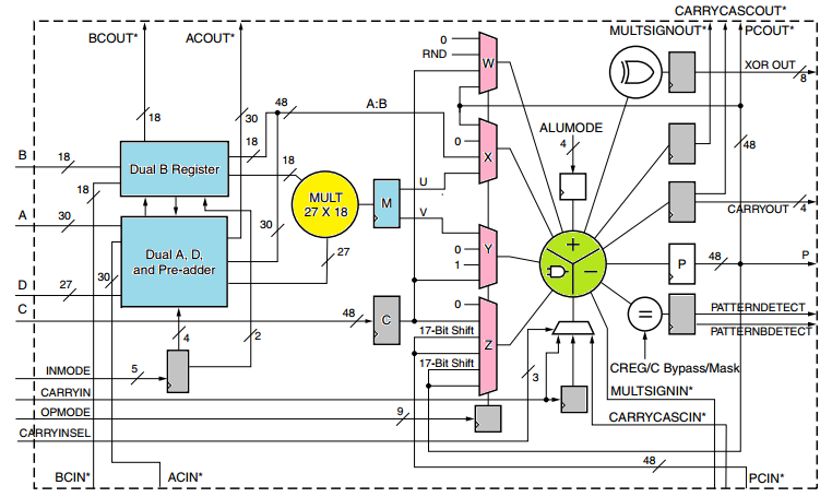
Bit depth coefficientsfor the described algorithm determines the frequency response unevenness in the passband and the obstacle band. In practice, the bit depth of the coefficients is set from 16 to 27 bits, which is associated with the features of the DSP48 node of modern FPGAs. For practical purposes, it is enough to set the bit depth of the coefficients to 16-18 bits and this will adequately provide the required uniformity of the frequency response. For high-order filters (for example, N = 256), a bit width of 18 bits is not enough and quantization effects begin to appear, in particular in the obstacle band. Therefore, for large-order filters, it is necessary to increase the bit depth of the coefficients, since the structure of the DSP48 processing nodes in the FPGA allows this (see Fig. DSP48 node).
Window filteringallows you to smooth out the ripple of the resulting frequency response in the passband after applying the filter corrector. The window function is superimposed on the impulse response of the calculated FIR filter (mathematically this is a convolution of spectra). Based on personal experience, I note that the Kaiser function is the best option for a window function. Using one BETA parameter, you can change the frequency response of the filter to the desired task. The Kaiser function is calculated through the modified zero-order Bessel functions I0 , but in many standard packages it is built-in ( Matlab, GNU Octave, MathCAD) Physically, the BETA parameter determines the fraction of energy concentrated within the main lobe of the spectrum. The higher the BETA parameter, the more concentrated the energy and the wider the main lobe, but the lower the level of the side lobes. For practical purposes, the parameter BETA = 3-11.
I will not give a detailed methodology for calculating the FIR filter; this can be read about in my previous article . There is nothing complicated - you need to obtain the FIR filter coefficients in any convenient way. You can do this using MathCAD, GNU Octave, Matlab (FDATool utility), ScopeFIR application, LabView program, or write your own calculation methodology based on well-known algorithms.
Algorithm
Let us describe the algorithm for calculating the correcting FIR filter. Below we will use the insertions of code in the Matlab scripting language for a better understanding of the implementation process.
1 step: we set the initial parameters of the CIC filter -
R = 8; % Decimation factor
N = 4; % Number of stages
M = 1; % Differential delay (only 1)
Step 2: we set the parameters of the FIR filter (bit depth of the coefficients, order, window) and the normalized cut-off frequency of the frequency response -
NFIR  = 128; % Filter order, must be odd when Fo = 0.5 !
Bc    = 16;  % Coef. Bit-width
Fo    = 0.3; % Normalized Cutoff: 0.2 < Fo < 0.5;
BETA  = 8;   % BETA parameter for Kaiser window (if IS_WIND = 'Y')
Step 3: Choose the step of "discretization" of vectors to calculate the characteristics. In accordance with this step, create the required arrays of numbers. We calculate the CIC filter according to the well-known formula and translate the result into decibels.
HCIC = (R^-N*abs(1*M*sin(pi*M*R*ff) ./ sin(pi*ff)).^N);
HCICdb = 20 * log10(abs(HCIC));
Step 4: In accordance with the effective bandwidth parameter Fo, we divide the vector of frequency samples into two parts: fp is the frequency vector in the passband, fs is the frequency vector in the attenuation band. We calculate the ideal characteristics of a compensating filter with a cutoff frequency Fo / R according to the following formula:

where f are samples of the normalized frequency in the bandwidth range from 0 to Fo / R. The remaining samples are zero.
% Calculate ideal response
Mp = ones(1, length(fp)); % Pass band response; Mp(1) = 1
Mp(2:end) = abs(M * R * sin(pi*fp(2:end)/R) ./ sin(pi*M*fp(2:end))).^(N);
Mf = [Mp zeros(1, length(fs))];
The type of the obtained characteristic is presented in the figure below:

Step 5: Using the ideal frequency response, we calculate the impulse response of the compensating FIR filter with the specified parameters (weight window, if any, bit depth of the coefficients and filter order).
Type of impulse response of the filter-corrector (calculation is performed using the built-in FIR2 function , and the window function is calculated through the FIR1 function ):
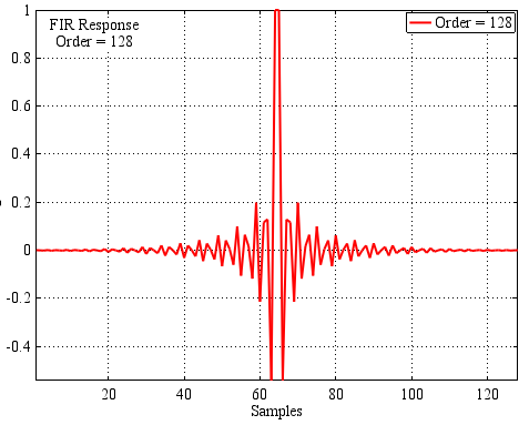
The source code for calculating their correction filter:
% Calculate FIR
hFIR = fir2(NFIR-1, f, Mf); % Filter length NFIR
hFIR = hFIR / max(hFIR); % Double coefficients
hCOE = round(hFIR*(2^(Bc-1)-1)); % Fixed point coefficients
% Windowed FIR (Kaiser with BETA)
if (IS_WIND == 'Y')
  WIND = kaiser(NFIR, BETA); % KAISER WINDOW IS USED!
  hWIND = fir1(NFIR-1, Fo/R, 'low', WIND);
  hNEW = hCOE .* hWIND;% conv2(hCOE,Hwind);
  hCOE = hNEW;
end
This completes the calculation of the filter. The result is a file of filter coefficients in a user-friendly way. As you can see, there is nothing complicated and the whole process is divided into 4-5 stages:
- Definition of input parameters of CIC and FIR filters,
- The formation of an ideal frequency response,
- Calculation of FIR filter coefficients ( FIR2 function ),
- The construction of the frequency response of the compensating filter for verification,
- Calculation of unevenness in the passband.
It should be noted that for circuits with a lower sampling frequency (decimation problem), compensating filters usually stand after CIC filters. For the tasks of increasing the sampling rate (interpolation), compensating filters stand before CIC filters. This arrangement of filters is best suited in terms of the amount of occupied crystal resources, since the FIR-correcting filter in this case operates at a lower frequency (after decimation or before interpolation).
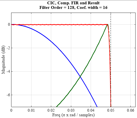
The following figure shows the frequency response of the CIC and FIR filters and the resulting frequency response after compensation for the following parameters:
- Decimation coefficient R = 11 ;
- CIC filter order N = 4 ;
- Delay in the circuit diff. link M = 1 ;
- The order of the FIR filter NFIR = 64 ;
- The capacity of the coefficients Bc = 16 ;
- Normalized cutoff frequency Fo = 0.4 ;
- Window function - not used

As you can see, the frequency response of the CIC filter is compensated, and the resulting frequency response visually has sufficient squareness (red curve).
Frequency response unevenness in the passband
Unfortunately, the alignment of the frequency response does not end there. Increase the graph within the bandwidth. In the next graph, you can see small beats in the strip.
Why is that? Frequency response in the passband is higher, the higher the order CIC-filter N . The decimation / interpolation coefficient R does not affect the unevenness. The irregularity is also affected by the order of the compensating FIR filter. The smaller the order of the filter, the greater the unevenness. But the greater the order of the filter, the greater the frequency of “beats” in the passband. For this reason, for practical purposes, high-order compensating filters NFIR> 128 are not used ! The effective band also makes an insignificant contribution: the smaller the alignment band, the less uneven.
To combat beats, window functions are used, which I spoke about earlier. Let's see what the graph looks like on an enlarged scale without window filtering and using the Kaiser function ( BETA = 8 ). Other parameters remain unchanged.

- Blue - the result without window filtering,
- Red - application of the Kaiser window function.
As you can see, window filtering allows you to smooth out the beats in the passband, making the resulting frequency response graph smooth.
The second way to improve the properties of the frequency response is to split the processing into several stages. For example, decimation is carried out not in one stage, but with the help of several links of lowering the sampling frequency: R = R1 * R2 * ... Rn .
In order to save FPGA resources in some tasks, it is possible to combine corrective and shaping FIR filters. To do this, you need to multiply their impulse characteristics or perform a convolution of the spectra.
Result
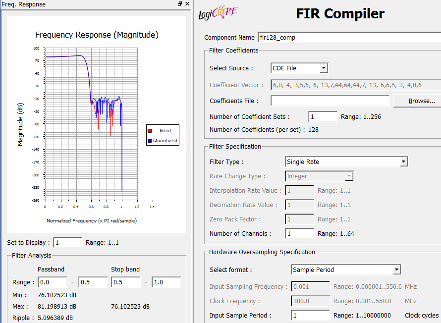
For the convenience of calculating the filter-corrector, an m-script has been written that allows you to get the result in a visual form. The script can display coefficient data in one of several popular formats, but you can add and modify it for your purposes if you wish.
- COE - Xilinx format for loading coefficients into Core Generator ,
- H - header file for connecting to C / C ++ projects (Code Composer Studio),

To run the script, you need Matlab or GNU Octave CAD software (I was debugging in the latter). Next, the resulting coefficient file is downloaded in * .COE format , to the Xilinx Core Generator, where a compensating FIR filter is implemented.
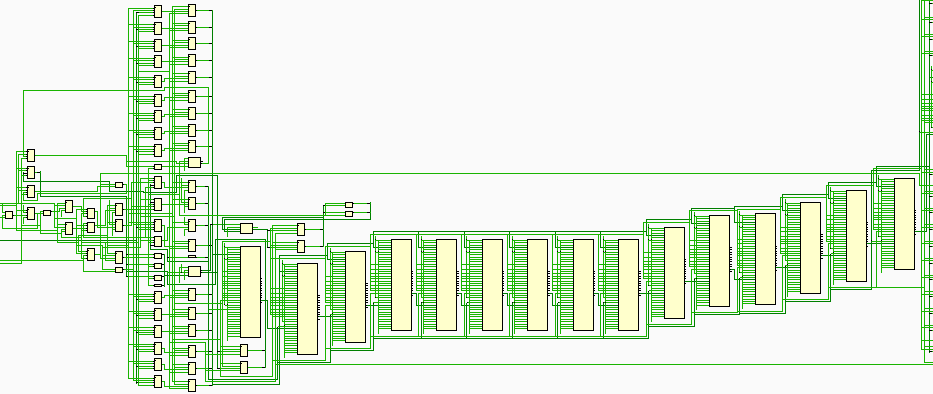
Schematic view of the FIR filter in Xilinx Vivado (post-synthesis tab):
Alternative method
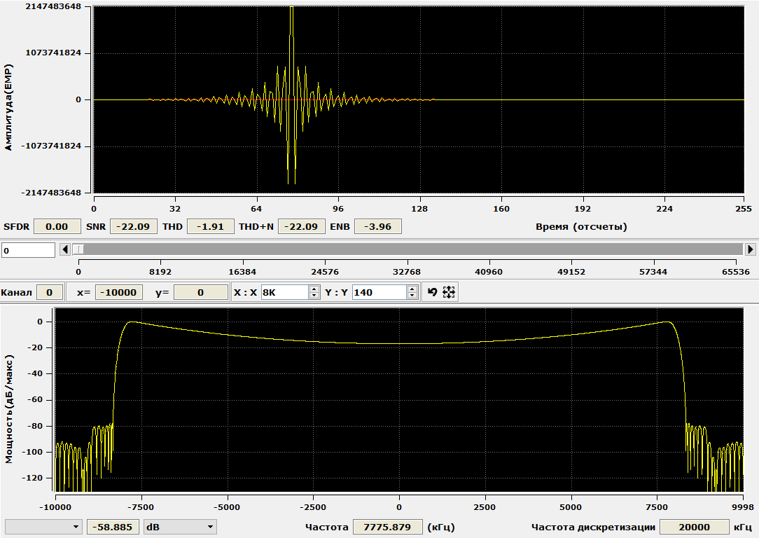
Another way to calculate corrective filters was suggested by my colleague at work - Antonov A.E. He wrote an interactive application that step by step in the manual mode selects the required non-uniformity of the frequency response of the filter and unloads the coefficients for further work. The proposed program, c_koeff.exe, is designed to correct the FIR filter coefficients behind a system of two CIC filters, to compensate for the uneven frequency response of the entire system in the passband introduced by the CIC filters. It is assumed that the FIR filter coefficients are obtained in the FDATool environment of the MATLAB package and are specified as a C-header file. The program is written in C ++ Builder. To display the calculated coefficients of the compensated FIR filter and its frequency response, the ISVI 6 program is usedand more, developed by InSys CJSC and distributed free of charge . In order not to violate the rules of the resource, I will not advertise the achievements of the company and the features of the applied software.
The result of the program is shown in the following figure. By enumerating the parameter Np , we obtain the spectral function of the compensating filter. In the ISVI application, you can also observe the impulse response of the filter.
The description of the application is in the word-file among the sources on github (link below).
Source
- m-scripts for Matlab / GNU Octave (calculation of FIR filters and correction filters)
- C_koeff application for interactive filter-corrector calculation
Literature
- Digital Signal Processing on FPGA - 1
- Digital Signal Processing on FPGA - 2
- Altera DS (Understanding CIC Compensation Filters)
- Using CIC filters in decimation and interpolation problems
- E.S. Eificher, Barry W. Dervis., Digital Signal Processing. Practical approach
- Rabiner L., Gold B., Theory and application of digital signal processing
- An economical class of digital filters for decimation and interpolation
Thanks for attention!