Fuzzy logic against PID. We cross a hedgehog and a snake. Aircraft engine and control algorithms for nuclear power plants

Probably, everyone who studied the theory of automatic control often had doubts about how these two, three or even ten squares of transfer functions in a model represent the dynamics of a complex unit, such as a nuclear reactor or an aircraft engine. Is there no cheating here? It is possible that working with simple models will cease to work with complex models and in "real" life.

In this article, we will experiment with the "real" model of an aircraft engine. Having weighed it with “real” models of equipment and control algorithms from a nuclear power plant.

Initially, the model was written in FORTRAN and is intended for some highly scientific purposes related to engine control systems. This model was given to us as an example and our task was to repeat the model in a structural form and prove that it coincides with the original one. What was done.

As soon as the model turned from listing Fortran into a structural scheme, it became easy and convenient to work with it, conducting any of the most "sophisticated" experiments. It was not by chance that I had real NPP control algorithms. That allowed us to quickly assemble a model for experiments, without using any formulas, yes, yes, only pictures.

Engine model

The model is a set of typical blocks that are configured to simulate the various components of a particular engine. In the previous article, we analyzed the gas turbine engine, in which the net power is removed using a shaft. In a turbojet engine, the net power is jet thrust, but we will be driving turns.

The general scheme of the model is shown in Figure 1.

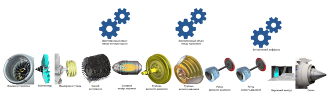
Figure 1. Schematic of the structural model of a turbojet engine.

Despite the fact that the model diagram looks like a scattering of three-dimensional parts, in reality it is a set of structural elements interconnected.

As an experiment, we, as in the previous article , will try to control the supply of fuel to obtain the desired speed.

For this we need a combustion chamber, in the properties of which we find the fuel consumption - that we will change. And in the parameters of the chamber there is an inlet pressure, which is calculated in this block. (see fig. 2 and 3)

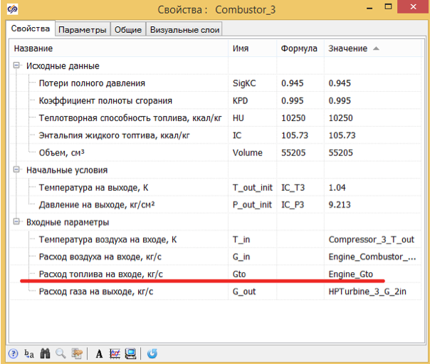
Figure 2. The properties of the combustion chamber.

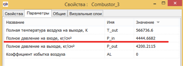
Figure 3. Combustion chamber parameters.

As an adjustable speed, take the speed of the low-pressure shaft. It seems to me that its revolutions have a more complicated dependence on the pressure of the fuel supply than the revolutions of the high-pressure shaft, which is affected by gases after the combustion chamber.

Fuel delivery model

In the original model, the fuel supply is specified in kg / s, as the boundary conditions for the simulation, as a tabular function of time. We want to create a model close to the “real” one, so we will use the proposal from the previous article and create a hydraulic model for the supply of fuel from the pipe and electro-valve.

As a model, we will define a pipe with a diameter of 10 mm, on which we will install an electric valve. The pressure on one side of the pipe is set constant, assuming that the fuel pump is working there. The pressure on the other side will be taken from the engine model. At the end of the pipe, add a narrowing of 2 times to simulate the nozzles. (Fig. 4)

Figure 4. Model of fuel supply to the engine.

The model is based on the dependence of the change in hydraulic resistance of the valve on the valve position.

This model will allow us to take into account the effect of pressure in the combustion chamber on fuel consumption, providing feedback. When we increase fuel consumption, pressure in the combustion chamber rises and, accordingly, the differential between the fuel pump and the combustion chamber decreases, which leads to a decrease in fuel consumption .

Pipeline costs are determined by solving a nonstationary fluid flow equation with allowance for friction, viscosity, density, and other physical effects, the description of which will take a couple - three pages of formulas.

Management model

To simulate a real control system, we will take a model of a regulator of steam supply to the turbine from the NPP control project. Not just the PID, which gives us the valve position, but an honest model in which there is:

1. Simulation of the drive motor operation taking into account the non-sensitivity zone, delays, opening and closing speeds.
2. FIR (impulse transformation relay) is a non-linear unit that provides for the conversion of a control action into the "open" and "close" commands.
3. PID regulator.
4. The inertia of the speed sensor.

To describe all the listed blocks and models, we will need another hundred hundred and fifty pages of text, so we will simply provide pictures with minimal explanations.

Valve model

It is a model of the engine and local control system.

The engine is a cunning integrator that processes the “open” and “close” commands, taking into account a given speed of movement of possible impacts, power failures, etc. (see fig. 5) At the outlet of this block, the valve position is calculated at each time point of the process simulation

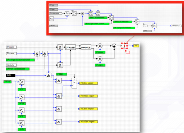
Figure 5. Motor Model

To control the valve motor, a valve control unit (COOK) is used, which provides logical processing of incoming commands and possible specified failures, as well as generates all the necessary signals for indication and control systems. (see fig. 6)

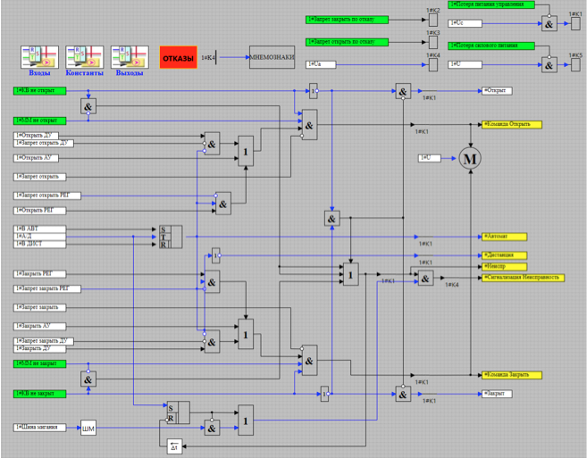
Figure 6. Model valve control unit (BEECH)

The schemes in Figures 5-6 are typical library schemes for simulating nuclear power plants. These blocks do not change the user, but are taken ready and used to create control algorithms. Control algorithms are created in the form of sheets. In our case, the sheet of the valve control algorithm is presented in Figure 7.

The direct formation of the “open” or “close” command (More, Less) is carried out in the relay pulse conversion unit (FIR). This unit can be executed both on “iron logic” (transistors, relays, amplifiers), and as a program.
The input of the FIR unit is the mismatch calculated by the PID unit as a percent deviation. The block itself, on the basis of these data, generates “open” or “close” pulses (more, less) for the valve control unit. The FIR block diagram is shown in Figure 8.

The algorithm of regulation of turns is presented on figure 9.

As the initial data for the calculation of the pressure regulator, the set value of turns and the sensor reading are used.

The PID algorithm itself is shown in Figure 10.

The speed sensor takes into account the delay, inertia and error of the real sensor. Diagram of the sensor model is shown in Figure 11.

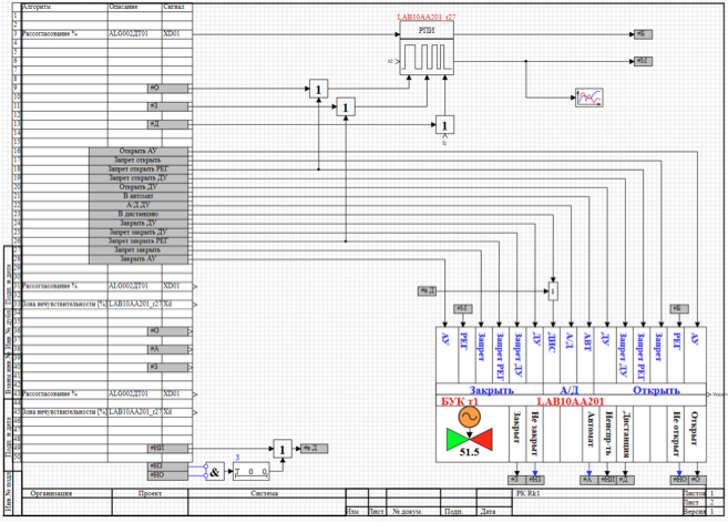
Figure 7. Valve Control Algorithm

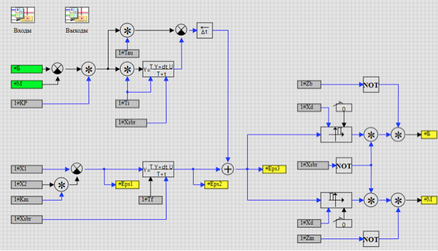
Figure 8. FIR block diagram

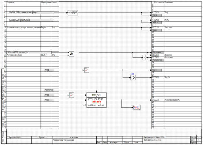
Figure 9. Controller Algorithm

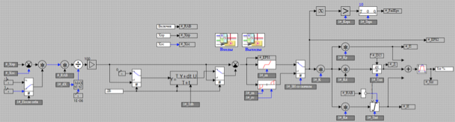
Figure 10. PID Controller

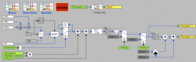
Figure 11. Sensor Model

As we see, the model is quite detailed (more than a thousand blocks) and is not linear at all.

Since in this experiment we explore the very possibility of optimizing and managing complex systems, the detail of the mathematical model is important for us, in terms of its nonlinearity and complexity. Therefore, such a “wild” combination of the real control program from the regulators of the nuclear power plant and the “real” model of the engine forms the task for testing the regulators with complex models.

• The control system uses the following settings:
• time of full opening and closing of the valve - 10 seconds
• engine speed control range - 1500 - 4000 rpm
• dead band for the regulator - 1%

Model setting and numerical experiment

The model we are investigating describes only the engine. And all the controls, such as fuel consumption, angles of rotation of the guide vane, flow rates, etc., are specified as functions that vary over time. We have created a “more honest” fuel supply model and are trying to connect it to the engine model. The numerical experiment plan is as follows:

1. bring the model of the engine to the nominal speed;
2. switch the fuel supply to the created control system;
3. to make regulation of turns.

Figure 12 shows the control scheme for conducting a numerical experiment.

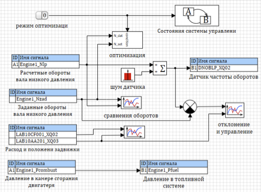
Figure 12. Numerical experiment control model

The model can operate in optimization mode or in control mode.

When the optimization mode is on, the optimization block works, in the off mode it does not participate in the calculation.

All models connected in a single package are considered synchronously exchanging data through the signal database. In the calculation management project, data is transferred from one model to another. In particular, the pressure from the engine's combustion chamber is transmitted to the pressure at the outlet of the fuel system, and the calculated low-pressure shaft revolutions are transmitted to the sensor model for consideration in the control system.

To simulate the inaccuracy of the measurement of revolutions, white noise is added to the calculated value of the revolutions of the shaft.

The specified turns are transferred to the optimization block. To control the quality of the transient process, flow and position graphs are used.

The control system is designed as a state machine with three states (see Fig. 13):

1. Acceleration engine. In this state, the engine model operates independently of the fuel system, and fuel consumption is specified as a piecewise linear function. The regulator is turned off, and the calculated low-pressure shaft turns are transferred to the set turns. Depending on the signal of the upper level, the transition can occur either to the optimization state or to the control state.
2. Optimization. In this state, fuel consumption is taken from the hydraulic model and transferred to the engine model. The PID controller is on and adjusts the valve position. The coefficients of the PID controller are taken from the optimization block and are applied to the controller in the optimization mode. The change in engine speed is given as a test effect.
3. Control. Exactly the same as optimization, except for the transfer of coefficients to the PID controller.

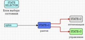
Figure 13. Motor control engine endpoints

Figure 14. States “Engine Acceleration” and “Optimization”

The adjustment of the regulator is carried out by the method of optimization. The optimization block diagram is shown in Figure 15. Depending on which control unit is used in the system for control, the optimization block selects values ​​for either the PID block or the fuzzy control block.

When setting the white noise is not taken into account (in the block is set as 0).

Figure 15. Regulator optimization block

Simulation results

The following process is used to select the PID controller coefficients:

Over 10 seconds, acceleration is performed using a pre-calculated fuel consumption curve. The frequency of rotation of the low pressure shaft at the end of acceleration is 3564 rpm.

At 10 seconds, the state machine switches over. From this point on, fuel consumption is taken from the hydraulic model, and the set frequency for the regulator is 3600 rpm.

At the 20th second of the calculation, the preset frequency changes - 3900 rpm.

Thus, the regulator must work out a step of 36 rpm at 10 seconds of the calculation and a step of 300 rpm at 30 seconds of the calculation.

The adjusted PID controller successfully copes with this task, taking into account the fact that at 10 seconds, besides the jump in revolutions, there is also a jump in fuel consumption at the moment of switching to the hydraulic model (see Fig. 16)

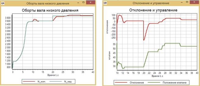
Figure 16. Revolutions and control processes for the PID controller

To create a controller based on fuzzy logic and purity of the experiment, we use the same PID controller already configured (see Fig. 10) to which we add a model of a controller based on fuzzy logic and replace the controller output - instead of a PID, we receive a signal obtained in fuzzy logic .

Thus, all the other parameters associated with normalization, the zone of inactivity, the work of the FIR remain the same as for the FID.

The output of the regulator, the same as the output for the FID, is the percentage mismatch.
And we left the PID regulator itself so that we can compare which impacts are given by the regulators. (see fig. 17)

Figure 17. PID Transformation in Fuzzy Logic

The regulator itself looks the same as in the first article . (see figure 18). The input is the mismatch, the first and second derivatives of the mismatch are determined numerically and a simple base of three rules is used:

• If less and decreases and slows down => decrease.
• If the rate and is constant and does not change => no change .
• If more and increases and accelerate => increase .

Figure 18. Diagram of a fuzzy regulator.

For tuning, we use the same variables that were used in the first article — these are the deviation ranges of the first and second derivatives of the deviation.

After optimization, we start the same transition process.

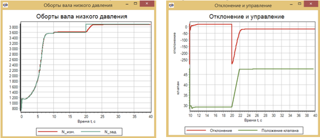
Figure 19. Turns and controls for fuzzy logic
The controller on fuzzy logic coped perfectly. Please note that the position of the valve at us "by itself" formed steps, when the valve stopped, paused and then moved again.

Judging from schedule 19, fuzzy logic coped much better with the increase in engine engine speed!

Now we will change the conditions of the task, which are set to a positive step of 300 rpm, and experience a negative step of -1500 rpm. (If we take more, the valve can close, but I don’t know how the model behaves at zero fuel consumption, although the real engine allows a short-term fuel supply.)

At 20 seconds, we set the frequency equal to 2100 rpm. And let's see how our regulators will work. The first in the ring - Fuzzy Logic.

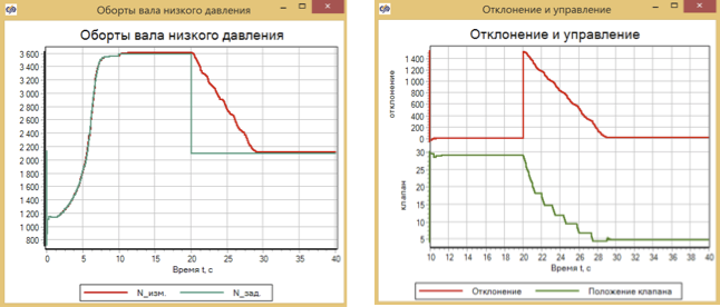
Figure 20. Testing the reduction of speed. Fuzzy logic

The second experiment is with the PID controller. And what do we see? This is a complete failure, the PID regulator, tuned to increase the frequency of revolutions, did not cope with a decrease in frequency. (see 21) Something anxiously became for me now for our nuclear power plants.

The engine model at low revs was absolutely uncontrollable with the help of a PID regulator tuned to control at high revs.

By the way, it can be seen that a brief shutdown of the fuel supply (the valve closes completely) does not lead to the collapse of the model of a turbojet engine.

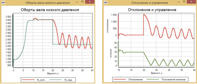
Figure 21. The development of reduced speed. PID regulator.

A test with a traffic controller is suggested, which uses the second derivative. Since such a model has already been made to the previous article (see Fig. 22), then converting fuzzy logic into traffic rules is a matter of two seconds. (see fig. 23).

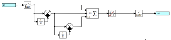
Figure 22. Block diagram of the PDA controller.

Figure 23. Replacing the PID on the traffic rules in the control algorithm

We carry out the adjustment of the regulator by the method of optimization and repeat the reduction in speed.

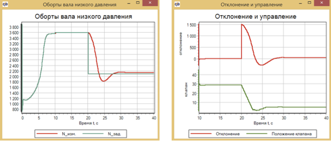
Figure 24 Testing the reduction in speed of traffic control regulator

The SDA worked with overshoot, but clearly better than PID, and almost as good as fuzzy logic. But there is an overshoot!

Complicate the task - add noise to the sensor

Now let's try to add white noise to the signal measurement sensor and see how the regulators behave with a real sensor. The dead zone we have 1% of the maximum speed - it is 40 rev / min. Set the white noise to 50 rpm.

Since the PID does not work at lower revs, we will test for increases.

The traffic controller obviously does not cope with such noises, although it maintains the required speed, but the control valve shakes, as in the dance of St. Vitus, when the given speed stands. In Figure 25, a specially extended section 25 - 26 seconds of the process

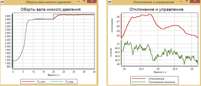
Figure 25 Speed ​​increase with sensor noise. Traffic regulator

Figure 26 Speed ​​increase with sensor noise. PID controller

The transition process for the PID controller has not changed despite the noise in the speed sensor. Management comes with clear and long steps.

The alarm for the nuclear power plant receded.

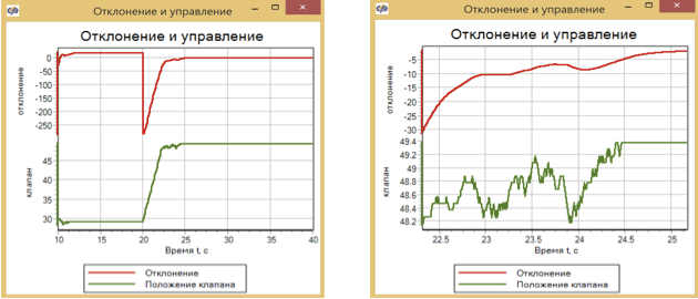
Figure 27. Fuzzy controller with noise in the sensor.

The controller with fuzzy logic with noise also controls, but at the moments of application to the stationary state, fluctuations in the position of the regulator occur.

findings

The third series of tests of fuzzy logic against PID and traffic rules ended with the victory of fuzzy logic. In contrast to the simple model of the previous article .

It was impossible to control the PID controller at low revs.

The experimentally detected PID advantage is the absence of oscillations in the case of a noisy sensor.

By the way, the dynamics of the engine (overclocking schedule) turned out to be very similar to the dynamics of the simplified model.

An archive with models for self-study can be found here.