At the very heart of the Meltwater and Fairhair.ai search engines is Elasticsearch, a collection of clusters with billions of media and social media articles.

Index shards in clusters vary greatly in access structure, workload, and size, which raises some very interesting problems.

In this article, we will describe how we used linear programming (linear optimization) to distribute the search and indexing workload as evenly as possible across all nodes in the clusters. This solution reduces the likelihood that one node will become a bottleneck in the system. As a result, we increased search speed and saved on infrastructure.

Background

Fairhair.ai's search engines contain about 40 billion social media and editorial posts, processing millions of queries daily. The platform provides customers with search results, graphs, analytics, data export for more advanced analysis.

These massive datasets reside in several 750-node Elasticsearch clusters with thousands of indexes in over 50,000 shards.

For more information about our cluster, see previous articles on its architecture and machine learning load balancer .

Uneven workload distribution

Both our data and user queries are usually date-bound. Most requests fall into a certain period of time, for example, last week, last month, last quarter or an arbitrary range. To simplify indexing and queries, we use time indexing , similar to the ELK stack .

Such an index architecture provides several advantages. For example, you can perform efficient mass indexing, as well as delete entire indexes when data is obsolete. It also means that the workload for a given index varies greatly over time.

Exponentially more queries go to the latest indexes, compared to the old ones.


Fig. 1. Access scheme for time indices. The number of completed queries is plotted on the vertical axis, and the index age is on the horizontal axis. Weekly, monthly, and annual plateaus are clearly visible, followed by a long tail of lower workload on older indices.

Patterns in Fig. 1 were quite predictable, as our customers are more interested in fresh information and regularly compare the current month with the past and / or this year with the past year. The problem is that Elasticsearch is unaware of this pattern and does not automatically optimize for the observed workload!

The built-in Elasticsearch shard allocation algorithm takes into account only two factors:

1. The number of shards on each node. The algorithm tries to evenly balance the number of shards per node throughout the cluster.
2. Labels free disk space. Elasticsearch considers the available disk space on a node before deciding whether to allocate new shards to this node or move segments from this node to others. With 80% of the used disk, it is forbidden to place new shards on a node, 90% of the system will begin to actively transfer shards from this node.

The fundamental assumption of the algorithm is that each segment in the cluster receives approximately the same amount of workload and that everyone has the same size. In our case, this is very far from the truth.

Standard load balancing quickly leads to hot spots in the cluster. They appear and disappear randomly, as the workload changes over time.

A hot spot is, in fact, a host operating near its limit of one or more system resources, such as a CPU, disk I / O, or network bandwidth. When this happens, the node first queues the requests for a while, which increases the response time to the request. But if the overload lasts a long time, then ultimately the requests are rejected, and users get errors.

Another common consequence of congestion is the unstable pressure of the JVM garbage due to queries and indexing operations, which leads to the “scary hell” phenomenon of the JVM garbage collector. In this situation, the JVM either can’t get the memory fast enough and crashes out of memory, or gets stuck in an endless garbage collection cycle, freezes and stops responding to requests and pings of the cluster.

The problem worsened when we refactored our architecture under AWS . Previously, we were “saved” by the fact that we ran up to four Elasticsearch nodes on our own powerful servers (24 cores) in our data center. This masked the influence of the asymmetric distribution of shards: the load was largely smoothed by a relatively large number of cores on the machine.

After refactoring, we placed only one node at a time on less powerful machines (8 cores) - and the first tests immediately revealed big problems with the “hot spots”.

Elasticsearch assigns shards in random order, and with more than 500 nodes in a cluster, the likelihood of too many “hot” shards on a single node has greatly increased - and such nodes have quickly overflowed.

For users, this would mean a serious deterioration in work, since congested nodes respond slowly, and sometimes completely reject requests or crash. If you bring such a system into production, then users will see frequent, it would seem, random UI slowdowns and random timeouts.

At the same time, there remains a large number of nodes with shards without much load, which are actually inactive. This leads to inefficient use of our cluster resources.

Both problems could be avoided if Elasticsearch distributed shards more intelligently, since the average use of system resources at all nodes is at a healthy level of 40%.

Cluster Continuous Change

When working more than 500 nodes, we observed one more thing: a constant change in the state of nodes. Shards constantly move back and forth in nodes under the influence of the following factors:

• New indexes are created, and old ones are discarded.
• Disk labels are triggered due to indexing and other shard changes.
• Elasticsearch randomly decides that there are too few or too many shards on the node compared to the average value of the cluster.
• Hardware crashes and crashes at the OS level cause new AWS instances to start and join them to the cluster. With 500 nodes, this happens on average several times a week.
• New sites are added almost every week due to normal data growth.

With all this in mind, we came to the conclusion that a complex and continuous solution to all problems requires a continuous and dynamic re-optimization algorithm.

Solution: Shardonnay

After a long study of the available options, we came to the conclusion that we want:

1. Build your own solution. We did not find any good articles, code, or other existing ideas that would work well on our scale and for our tasks.
2. Launch the rebalancing process outside of Elasticsearch and use the clustered redirect APIs rather than trying to create a plugin . We wanted a quick feedback loop, and deploying a plugin on a cluster of this magnitude could take several weeks.
3. Use linear programming to calculate the optimal shard movements at any given time.
4. Perform optimization continuously so that the cluster state gradually comes to the optimum.
5. Do not move too many shards at the same time.

We noticed an interesting thing: if you move too many shards at the same time, it is very easy to trigger a cascading storm of shard movement . After the onset of such a storm, it can continue for hours, when shards uncontrollably move back and forth, causing the appearance of marks about the critical level of disk space in various places. In turn, this leads to new shard movements and so on.

To understand what is happening, it is important to know that when you move an actively indexed segment, it actually begins to use much more space on the disk from which it is moving. This is due to how Elasticsearch saves transaction logs.. We saw cases when the index doubled when moving the node. This means that the node that initiated the shard movement due to high disk space usage will use even more disk space for a while until it moves enough shards to other nodes.

To solve this problem, we developed the Shardonnay service in honor of the famous Chardonnay grape variety.

Linear optimization

Linear optimization (or linear programming , LP) is a method of achieving the best result, such as maximum profit or lowest cost, in a mathematical model whose requirements are represented by linear relationships.

The optimization method is based on a system of linear variables, some constraints that must be met, and an objective function that determines what a successful solution looks like. The goal of linear optimization is to find the values ​​of variables that minimize the objective function, subject to restrictions.

Shard distribution as a linear optimization problem

Shardonnay should work continuously, and at each iteration it performs the following algorithm:

1. Using the API, Elasticsearch retrieves information about existing shards, indexes, and nodes in the cluster, as well as their current location.
2. Models the state of a cluster as a set of binary LP variables. Each combination (node, index, shard, replica) gets its own variable. In the LP model, there are a number of carefully designed heuristics, restrictions, and an objective function, more on this below.
3. Sends the LP model to a linear solver, which gives an optimal solution taking into account the constraints and the objective function. The solution is to reassign shards to nodes.
4. Interprets the LP solution and converts it into a sequence of shard movements.
5. Instructs Elasticsearch to move shards through the cluster redirect API.
6. Waits for the cluster to move the shards.
7. Returns to step 1.

The main thing is to develop the right constraints and objective function. The rest will be done by Solver LP and Elasticsearch.

Not surprisingly, the task was very difficult for a cluster of this size and complexity!

Limitations

We base some restrictions on the model based on the rules dictated by Elasticsearch itself. For example, always stick to disk labels or prohibit placing a replica on the same node as another replica of the same shard.

Others are added based on experience gained over years of working with large clusters. Here are some examples of our own limitations:

• Do not move today's indexes, as they are the hottest and get an almost constant load on reading and writing.
• Give preference to moving smaller shards, because Elasticsearch handles them faster.
• It is advisable to create and place future shards a few days before they become active, begin to be indexed, and undergo a heavy load.

Cost function

Our cost function weighs together a number of different factors. For example, we want:

• minimize the variance of indexing and search queries in order to reduce the number of "hot spots";
• keep the minimum dispersion of disk usage for stable system operation;
• minimize the number of shard movements so that "storms" with a chain reaction do not begin, as described above.

Reduction of drug variables

On our scale, the size of these LP models becomes a problem. We quickly realized that problems could not be solved in a reasonable time with more than 60 million variables. Therefore, we applied many optimization and modeling tricks to drastically reduce the number of variables. Among them are biased sampling, heuristics, the divide and conquer method, iterative relaxation and optimization. Fig. 2. The heat map shows the unbalanced load on the Elasticsearch cluster. This is manifested in a large dispersion of resource use on the left side of the graph. Through continuous optimization, the situation is gradually stabilizing . 3. The heat map shows the CPU usage on all nodes of the cluster before and after setting up the hotness function in Shardonnay. A significant change in CPU utilization is seen with constant workload.








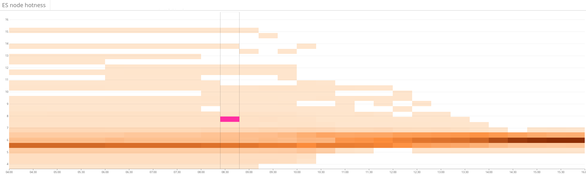
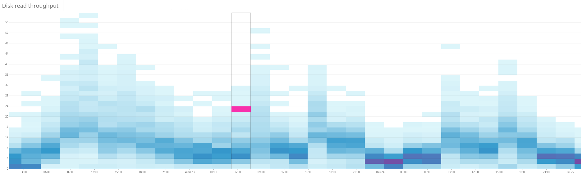
Fig. 4. The heat map shows the read throughput of the disks during the same period as in fig. 3. Read operations are also more evenly distributed across the cluster.

results

As a result, our LP solver finds good solutions in a few minutes, even for our huge cluster. Thus, the system iteratively improves the state of the cluster in the direction of optimality.

And the best part is that the variance of the workload and disk usage converges as expected - and this near-optimal state is maintained after many intentional and unexpected changes in the cluster state since!

We now support healthy workload distribution in our Elasticsearch clusters. All thanks to linear optimization and our service, which we love call Chardonnay .