Visualization of static and dynamic networks on R, part 2
- Transfer
- Tutorial
In the first part :
In this part: colors and fonts in R. charts.
Colors are beautiful, but more importantly, they help to distinguish between types of objects, gradations of properties. Most R functions can use color names , RGB, or hexadecimal values . In a simple basic graph, R is below

As you can see, RGB here varies from 0 to 1. This is the default setting for R, but you can also set the range from 0 to 255 using the command
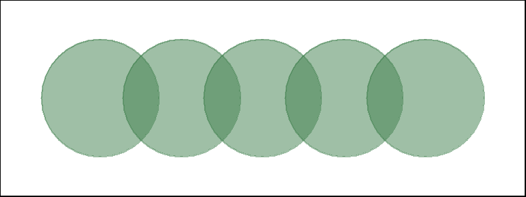
You can set the transparency of an element using the parameter
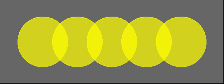
If you are using a hexadecimal color representation, you can set the opacity using
If you plan to use the built-in color names, here's how to get them all:
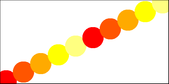
In most cases, we need either several contrasting colors, or shades of the same color. R has a built-in palette function that can generate this. For instance:

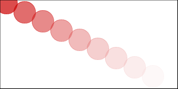
We can also create our own gradients with

To add transparency to
Finding a good combination of colors is not an easy task, while the built-in R palettes are quite limited. Fortunately, other packages solve this problem:
There is one main function in this package -


Using palettes

Using different fonts in R graphs may require some effort. This is especially true for Windows users, Mac and Linux users are likely to safely skip this section.
In order to import fonts from the OS into R, we use the package
Fonts are now available, and you can do something like this:
When you save graphics as PDF files, you can also install fonts:
- network visualization: why? how?
- visualization options
- best practices - aesthetics and performance
- data formats and preparation
- description of the data sets used in the examples
- getting started with igraph
In this part: colors and fonts in R. charts.
Brief Introduction I: Colors in R Charts
Colors are beautiful, but more importantly, they help to distinguish between types of objects, gradations of properties. Most R functions can use color names , RGB, or hexadecimal values . In a simple basic graph, R is below
xand y- the coordinates of the points, pch- the symbol for the points, cex- the size of the point and col- the color. To find out what are the options for plotting in R, run the command ?par.plot(x=1:10, y=rep(5,10), pch=19, cex=3, col="dark red")
points(x=1:10, y=rep(6, 10), pch=19, cex=3, col="557799")
points(x=1:10, y=rep(4, 10), pch=19, cex=3, col=rgb(.25, .5, .3))
As you can see, RGB here varies from 0 to 1. This is the default setting for R, but you can also set the range from 0 to 255 using the command
rgb(10, 100, 100, maxColorValue=255). You can set the transparency of an element using the parameter
alpha(from 0 to 1):plot(x=1:5, y=rep(5,5), pch=19, cex=12, col=rgb(.25, .5, .3, alpha=.5), xlim=c(0,6))
If you are using a hexadecimal color representation, you can set the opacity using
adjustcolorthe package grDevices. For the sake of interest, we will also paint the background of the graph in gray using the function par()to set the graphics settings.par(bg="gray40")
col.tr <- grDevices::adjustcolor("557799", alpha=0.7)
plot(x=1:5, y=rep(5,5), pch=19, cex=12, col=col.tr, xlim=c(0,6))
If you plan to use the built-in color names, here's how to get them all:
colors()                          # List all named colors
grep("blue", colors(), value=T)   # Colors that have "blue" in the name
In most cases, we need either several contrasting colors, or shades of the same color. R has a built-in palette function that can generate this. For instance:
pal1 <- heat.colors(5, alpha=1)   #  5 colors from the heat palette, opaque
pal2 <- rainbow(5, alpha=.5)      #  5 colors from the heat palette, transparent
plot(x=1:10, y=1:10, pch=19, cex=5, col=pal1)
plot(x=1:10, y=1:10, pch=19, cex=5, col=pal2)
We can also create our own gradients with
colorRampPalette. Note that it colorRampPalettereturns a function that can be used to generate as many colors from this palette as needed.palf <- colorRampPalette(c("gray80", "dark red"))
plot(x=10:1, y=1:10, pch=19, cex=5, col=palf(10))
To add transparency to
colorRampPalette, you need to use the parameter alpha=TRUE:palf <- colorRampPalette(c(rgb(1,1,1, .2),rgb(.8,0,0, .7)), alpha=TRUE)
plot(x=10:1, y=1:10, pch=19, cex=5, col=palf(10))
Finding a good combination of colors is not an easy task, while the built-in R palettes are quite limited. Fortunately, other packages solve this problem:
# If you don't have R ColorBrewer already, you will need to install it:
install.packages("RColorBrewer")
library(RColorBrewer)
display.brewer.all()
There is one main function in this package -
brewer.pal. In order to use it, you only need to select the necessary palette and the number of colors. Let's take a look at some palettes RColorBrewer:display.brewer.pal(8, "Set3")
display.brewer.pal(8, "Spectral")
display.brewer.pal(8, "Blues")
Using palettes
RColorBrewerin graphs:pal3 <- brewer.pal(10, "Set3")
plot(x=10:1, y=10:1, pch=19, cex=4, col=pal3)
Brief Introduction II: Fonts in R Charts
Using different fonts in R graphs may require some effort. This is especially true for Windows users, Mac and Linux users are likely to safely skip this section.
In order to import fonts from the OS into R, we use the package
extrafont:install.packages("extrafont")
library(extrafont)
# Import system fonts - may take a while.
font_import()
fonts() # See what font families are available to you now.
loadfonts(device = "win") # use device = "pdf" for pdf plot output.
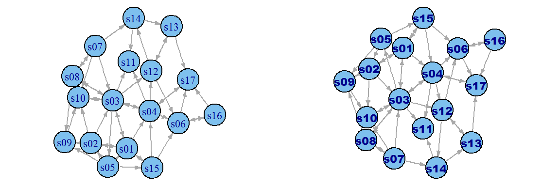
Fonts are now available, and you can do something like this:
library(extrafont)
plot(net, vertex.size=30)
plot(net, vertex.size=30, vertex.label.family="Arial Black" )
When you save graphics as PDF files, you can also install fonts:
# First you may have to let R know where to find ghostscript on your machine:
Sys.setenv(R_GSCMD = "C:/Program Files/gs/gs9.10/bin/gswin64c.exe")
# pdf() will send all the plots we output before dev.off() to a pdf file:
pdf(file="ArialBlack.pdf")
plot(net, vertex.size=30, vertex.label.family="Arial Black" )
dev.off()
embed_fonts("ArialBlack.pdf", outfile="ArialBlack_embed.pdf")