Molecular Dynamics Programming
Good time of the day hawkers and hawkers. Today I would like to share with you my attempts at programming physical processes. More specifically, an attempt to delve into molecular proportions. The topic of conversation under the habrakat is molecular dynamics.
As Wikipedia says , MD is a method in which the temporal evolution of a system of interacting atoms or particles is tracked by integrating their equations of motion.
If it’s even simpler, we set the initial conditions (velocities, positions of particles, their type) and knowing the laws of their interaction, we look what will come of it. It reminds me of the good old Live game.
Everything is very simple here. The interactions between particles (in my particular case, atoms) will be considered using classical physics:

This seemingly confusing formula is actually a complete analog of school F = ma.
(in fact, the “entangled” formula is longer, and looks less aesthetically pleasing - I deliberately forgot the dissipative component)
Mathematically, particle modeling is a solution to the Cauchy problem for the equations above.
The calculation of this whole thing, I entrusted the Verlet algorithm.
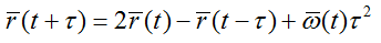
IMHO, it is optimal in accuracy and speed. One thing - he needs to know the two previous positions of the particle! Therefore, the first step is left to inaccurate Euler.
Ф (r) in the formula above is determined through the potential. In general, the potential here is the king and god - it is precisely his influence that is most significant. I chose a pretty popular - get acquainted, Lennard-Jones:
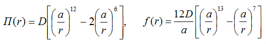
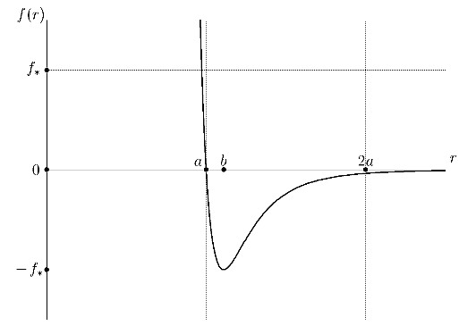
And this is how it looks here as it is the interatomic distance, f - force interaction, r - distance between the particles.
Let's move on to programming. Having scored all this in the code, we get arrays of accelerations and coordinates at the output (oh yes, Verle does not operate with speeds, speeds can be obtained, for example, using central differences). The visualization of all this stuffing I, not particularly bothering, instructed OpenGL.
Let’s look at the spall (1083 particles, the drummer “falls” onto the target)


This is exactly the moment, perhaps the most pleasant - to play with a fresh model. Only the low calculation speed depressed - the time for optimizations has come.
First of all, I had to return to physics. Only one look at the potential made it clear - with a radius greater than 2a - we can not count. Those. the easiest way is for each particle to consider interaction only with particles falling into a sphere of radius a2 with a center in the particle for which we assume. One condition is “if” and the calculation is accelerated several times (depending on the number of particles and region).
Watching the full load of one core on my hospital is a dull task. It’s time to parallelize the process. Especially since md perfectly parallels. It would seem simple - set the correspondence: the particle is the processor and count. Practice has shown - it’s better to parallelize, breaking the space into a grid and that’s why.
By creating a grid with a cell size equal to a, we kill two birds with one stone - we solve the problem with the calculation area, where the interaction is taken into account and we make the exchange between processors more transparent and simple. Here's what it looks like on the example of two processors:

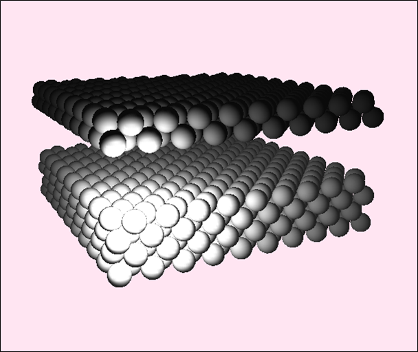
Here it’s worth mentioning that any model is also “chased” by various “hacks” depending on the initial conditions. For example, if we need to model something infinite (or huge) and at the same time have the same structure in one or several directions, we can apply periodic boundary conditions. I used this to simulate the friction of two infinite surfaces.
The point here is that around its computational domain its “images” are built, with the actual position of the particles. And the particles of the “real” region interact with the particles in the “image”. And if a particle crosses the boundary of the computational domain, it appears on the other side (aka tunnel in pacman). The following is an example of periodic conditions for x and y.
But to simulate friction, I used periodicals on only one axis:


It turned out to be a rather interesting and intuitive model, which is quite possible to both play and try to use it for real calculation (the reliability of the results is very decent). For a good application, it would be worth sharpening under Cuda or OpenCL - the speed of calculating the MD on video cards, with proper parallelization, is simply prohibitive! However, betting on your laziness - soon this is unlikely to happen.
PS: For the most part, I relied on only one book: The Particle Method and its Use in the Mechanics of Deformable Solid Case. Krivtsov A.M., Krivtsova N.V.
What is MD?
As Wikipedia says , MD is a method in which the temporal evolution of a system of interacting atoms or particles is tracked by integrating their equations of motion.
If it’s even simpler, we set the initial conditions (velocities, positions of particles, their type) and knowing the laws of their interaction, we look what will come of it. It reminds me of the good old Live game.
Maths
Everything is very simple here. The interactions between particles (in my particular case, atoms) will be considered using classical physics:
This seemingly confusing formula is actually a complete analog of school F = ma.
(in fact, the “entangled” formula is longer, and looks less aesthetically pleasing - I deliberately forgot the dissipative component)
Mathematically, particle modeling is a solution to the Cauchy problem for the equations above.
The calculation of this whole thing, I entrusted the Verlet algorithm.
IMHO, it is optimal in accuracy and speed. One thing - he needs to know the two previous positions of the particle! Therefore, the first step is left to inaccurate Euler.
Without potential anywhere
Ф (r) in the formula above is determined through the potential. In general, the potential here is the king and god - it is precisely his influence that is most significant. I chose a pretty popular - get acquainted, Lennard-Jones:
And this is how it looks here as it is the interatomic distance, f - force interaction, r - distance between the particles.
Enough formulas
Let's move on to programming. Having scored all this in the code, we get arrays of accelerations and coordinates at the output (oh yes, Verle does not operate with speeds, speeds can be obtained, for example, using central differences). The visualization of all this stuffing I, not particularly bothering, instructed OpenGL.
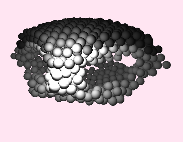
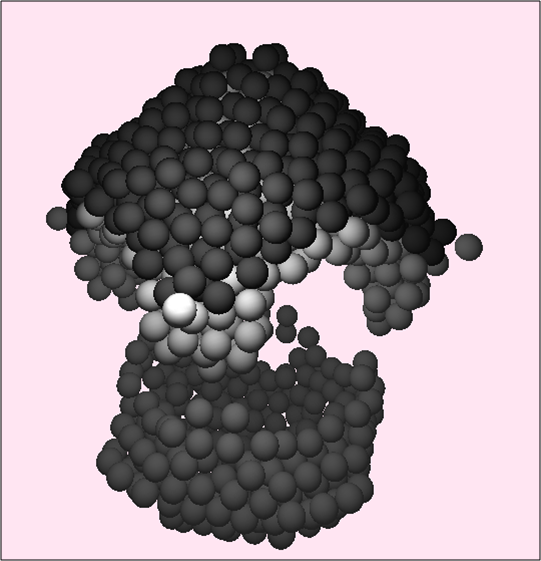
Let’s look at the spall (1083 particles, the drummer “falls” onto the target)
This is exactly the moment, perhaps the most pleasant - to play with a fresh model. Only the low calculation speed depressed - the time for optimizations has come.
Speed up
First of all, I had to return to physics. Only one look at the potential made it clear - with a radius greater than 2a - we can not count. Those. the easiest way is for each particle to consider interaction only with particles falling into a sphere of radius a2 with a center in the particle for which we assume. One condition is “if” and the calculation is accelerated several times (depending on the number of particles and region).
Watching the full load of one core on my hospital is a dull task. It’s time to parallelize the process. Especially since md perfectly parallels. It would seem simple - set the correspondence: the particle is the processor and count. Practice has shown - it’s better to parallelize, breaking the space into a grid and that’s why.
By creating a grid with a cell size equal to a, we kill two birds with one stone - we solve the problem with the calculation area, where the interaction is taken into account and we make the exchange between processors more transparent and simple. Here's what it looks like on the example of two processors:
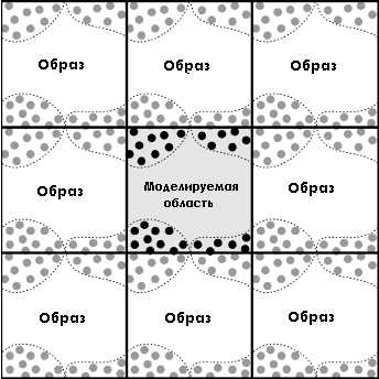
Here it’s worth mentioning that any model is also “chased” by various “hacks” depending on the initial conditions. For example, if we need to model something infinite (or huge) and at the same time have the same structure in one or several directions, we can apply periodic boundary conditions. I used this to simulate the friction of two infinite surfaces.
The point here is that around its computational domain its “images” are built, with the actual position of the particles. And the particles of the “real” region interact with the particles in the “image”. And if a particle crosses the boundary of the computational domain, it appears on the other side (aka tunnel in pacman). The following is an example of periodic conditions for x and y.
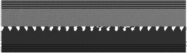
But to simulate friction, I used periodicals on only one axis:
Conclusion
It turned out to be a rather interesting and intuitive model, which is quite possible to both play and try to use it for real calculation (the reliability of the results is very decent). For a good application, it would be worth sharpening under Cuda or OpenCL - the speed of calculating the MD on video cards, with proper parallelization, is simply prohibitive! However, betting on your laziness - soon this is unlikely to happen.
PS: For the most part, I relied on only one book: The Particle Method and its Use in the Mechanics of Deformable Solid Case. Krivtsov A.M., Krivtsova N.V.