About degrees of freedom in statistics
In a previous post, we discussed perhaps the central concept in data analysis and hypothesis testing - the p-level of significance. If we do not use the Bayesian approach, then we use the p-value to decide whether we have enough reason to reject the null hypothesis of our study, i.e. proudly tell the world that we have obtained statistically significant differences.
However, in most statistical tests used to test hypotheses (for example, t-test, regression analysis, analysis of variance), next to p-value is always adjacent to such an indicator as the number of degrees of freedom, it is also degrees of freedom or simply abbreviated df, about it we’ll talk today.

In my opinion, the concept of degrees of freedom in statistics is remarkable in that it is at the same time one of the most important in applied statistics (we need to know df for calculating p-value in the voiced tests), but at the same time it is one of the most difficult to understand definitions for non-math students studying statistics.
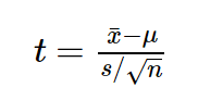
Let's look at an example of a small statistical study to understand why we need the df indicator, and what is the problem with it. Suppose we decided to test the hypothesis that the average growth of residents of St. Petersburg is 170 centimeters. For these purposes, we collected a sample of 16 people and obtained the following results: the average growth in the sample turned out to be 173 with a standard deviation of 4. To test our hypothesis, we can use the one-sample student t-test, which allows us to estimate how strongly the sample mean deviated from the expected average in the general population in units of standard error:
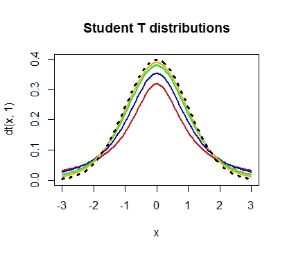
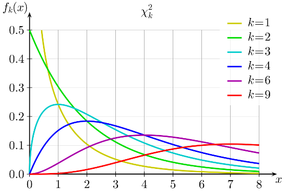
We will carry out the necessary calculations and find that the value of the t-criterion is 3, excellent, it remains to calculate the p-value and the problem is solved. However, having got acquainted with the features of the t-distribution, we find out that its shape varies depending on the number of degrees of freedom calculated by the formula n-1, where n is the number of observations in the sample:
The formula for calculating df itself looks very friendly, we substituted the number of observations, subtracted one and the answer is ready: it remains to calculate the p-value, which in our case is 0.004.
When for the first time in my life at a lecture on statistics I came across this procedure, like many students I had a legitimate question: why do we subtract one? Why don't we subtract the deuce, for example? And why should we subtract anything from the number of observations in our sample?
In the textbook, I read the following explanation, which I met more than once in the future as an answer to this question:
“Suppose we know what the sample average equals, then we need to know only n-1 sample elements in order to accurately determine what the remaining n element equals.” It sounds reasonable, but such an explanation rather describes some mathematical technique than explains why we needed to use it in calculating the t-criterion. The following common explanation is as follows: the number of degrees of freedom is the difference between the number of observations and the number of estimated parameters. When using the one-sample t-test, we estimated one parameter - the average value in the general population, using n sample elements, which means df = n-1.
However, neither the first nor the second explanation helps to understand why exactly we needed to subtract the number of estimated parameters from the number of observations?
Let's move a little further in search of an answer. First we turn to the definition of t-distribution, it is obvious that all the answers are hidden in it. So a random variable:
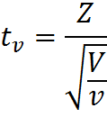
has a t-distribution with df = ν, provided that Z is a random variable with a standard normal distribution of N (0; 1), V is a random variable with a Chi-square distribution, with ν is the number of degrees of freedom, random variables Z and V are independent. This is a serious step forward; it turns out that the random variable with the Chi-square distribution in the denominator of our formula is responsible for the number of degrees of freedom.
Let’s then study the definition of the Chi-square distribution. A Chi-square distribution with k degrees of freedom is a distribution of the sum of squares of k independent standard normal random variables.
It seems that we are already quite on target, at least now we know for sure that such a number of degrees of freedom for the Chi-square distribution is just the number of independent random variables with a normal standard distribution that we summarize. But it still remains unclear at what stage and why we needed to subtract the unit from this value?
Let's look at a small example that clearly illustrates this need. Let's say we really like to make important life decisions based on the result of a coin toss. However, recently, we suspected our coin of having eagle too often. In order to try to reject the hypothesis that our coin is actually honest, we recorded the results of 100 throws and got the following result: the eagle fell 60 times and the tails fell only 40 times. Do we have enough reason to reject the hypothesis that the coin is fair? This will help us and the distribution of Chi-square Pearson. After all, if the coin was truly honest, then the expected, theoretical frequencies of the eagle and tails to fall would be the same, that is, 50 and 50. It is easy to calculate how much the observed frequencies deviate from the expected. To do this, we calculate the Pearson's Chi-square distance according to, I think, the formula familiar to most readers:
Where O are observable, E are expected frequencies.
The fact is that if the null hypothesis is true, then when our experiment is repeated many times, the distribution of the difference between the observed and expected frequencies, divided by the root of the observed frequency, can be described using the normal standard distribution, and this will be the sum of the squares k of such random normal values by definition, a random variable having a chi-square distribution.
Let's illustrate this thesis graphically, let's say we have two random, independent variables that have a standard normal distribution. Then their joint distribution will look as follows:
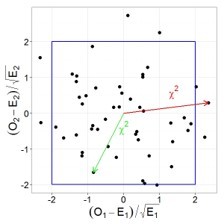
In this case, the square of the distance from zero to each point will be a random variable having a Chi-square distribution with two degrees of freedom. Recalling the Pythagorean theorem, it is easy to verify that this distance is the sum of the squares of the values of both quantities.
Well, now the culmination of our story. We return to our formula for calculating the Chi-square distance to check the integrity of the coin, substitute the available data in the formula and find that the Pearson Chi-square distance is 4. However, to determine the p-value, we need to know the number of degrees of freedom, because the shape of the Chi-square distribution depends on this parameter, respectively, and the critical value will also vary depending on this parameter.
Now the fun part. Suppose that we decided to repeat 100 throws many times, and each time we recorded the observed frequencies of eagles and tails, calculated the required indicators (the difference between the observed and expected frequencies, divided by the root of the expected frequency) and, as in the previous example, plotted them on a graph.
It is easy to see that now all the points are aligned in one line. The thing is that in the case of a coin, our terms are not independent, knowing the total number of throws and the number of tails, we can always accurately determine the dropped number of eagles and vice versa, therefore we cannot say that our two terms are two independent random quantities. You can also make sure that all points will always always lie on one straight line: if we had 30 eagles, then there were 70 tails, if 70 eagles, then 30 tails, etc. Thus, despite the fact that there were two terms in our formula, we will use the Chi-square distribution with one degree of freedom to calculate p-value! So we finally got to the moment when we needed to subtract the unit. If we tested the hypothesis that Since our dice with six faces is honest, we would use a Chi-square distribution with 5 degrees of freedom. After all, knowing the total number of throws and the observed frequency of loss of any five faces, we can always determine exactly what the number of drops of the sixth face equals.
Now, armed with this knowledge, back to the t-test:
we have the standard error in the denominator, which is the sample standard deviation divided by the root of the sample size. The calculation of the standard deviation includes the sum of the squares of the deviations of the observed values from their average value - that is, the sum of several random positive values. But we already know that the sum of the squares of n random variables can be described using the chi-square distribution. However, despite the fact that we have n terms, this distribution will have an n-1 degree of freedom, since knowing the sample average and n-1 elements of the sample, we can always precisely specify the last element (hence this explanation about the average and n-1 elements needed to uniquely identify n elements)! It turns out that in the denominator of t-statistics we have hidden the chi-square distribution with n-1 degrees of freedom, which is used to describe the distribution of the sample standard deviation! Thus, the degrees of freedom in the t-distribution are actually taken from the chi-square distribution, which is hidden in the t-statistic formula. By the way, it is important to note that all the above considerations are true if the trait under study has a normal distribution in the general population (or the sample size is large enough), and if we really had the goal of testing the hypothesis of the average value of growth in the population, perhaps it is more reasonable to use a nonparametric criterion.
A similar logic for calculating the number of degrees of freedom is preserved when working with other tests, for example, in regression or variance analysis, the thing is in random variables with the Chi-square distribution, which are present in the formulas for calculating the relevant criteria.
Thus, in order to correctly interpret the results of statistical studies and to understand where all the indicators that we get when using even such a simple criterion as a single-sample t-test arise, any researcher needs to understand well what mathematical ideas underlie statistical methods.
Based on the experience of teaching statistics at the Institute of Bioinformatics , we had the idea to create a series of online courses devoted to data analysis, in which the most important topics will be explained in an accessible form for each, understanding of which is necessary for the confident use of statistical methods in solving various problems. In 2015, we launched the Fundamentals of Statistics course , to which about 17 thousand people have signed up today, three thousand students have already received a certificate of successful completion, and the course itself has been awarded the EdCrunch Awards and recognized as the best technical course. This year, on the stepik.org platform , the continuation of the Basics of Statistics course has started . Part two, in which we continue our acquaintance with the basic methods of statistics and analyze the most complex theoretical issues. By the way, one of the main topics of the course is the role of the Pearson Chi-square distribution in testing statistical hypotheses. So if you still have questions about why we subtract the unit from the total number of observations, we are waiting for you on the course!
It is also worth noting that theoretical knowledge in the field of statistics will definitely be useful not only to those who use statistics for academic purposes, but also to those who use data analysis in applied fields. Basic knowledge of statistics is simply necessary to master the more complex methods and approaches that are used in the field of machine learning and Data Mining. Thus, successfully completing our introduction to statistics courses is a good start in data analysis. Well, if you are seriously thinking about acquiring data skills, we think you may be interested in our online data analysis program, which we wrote about in more detail here. The statistics courses mentioned are part of this program and will allow you to smoothly immerse yourself in the world of statistics and machine learning. However, everyone can take these courses without deadlines, even outside the context of a data analysis program.
However, in most statistical tests used to test hypotheses (for example, t-test, regression analysis, analysis of variance), next to p-value is always adjacent to such an indicator as the number of degrees of freedom, it is also degrees of freedom or simply abbreviated df, about it we’ll talk today.
Degrees of freedom, what are we talking about?
In my opinion, the concept of degrees of freedom in statistics is remarkable in that it is at the same time one of the most important in applied statistics (we need to know df for calculating p-value in the voiced tests), but at the same time it is one of the most difficult to understand definitions for non-math students studying statistics.
Let's look at an example of a small statistical study to understand why we need the df indicator, and what is the problem with it. Suppose we decided to test the hypothesis that the average growth of residents of St. Petersburg is 170 centimeters. For these purposes, we collected a sample of 16 people and obtained the following results: the average growth in the sample turned out to be 173 with a standard deviation of 4. To test our hypothesis, we can use the one-sample student t-test, which allows us to estimate how strongly the sample mean deviated from the expected average in the general population in units of standard error:
We will carry out the necessary calculations and find that the value of the t-criterion is 3, excellent, it remains to calculate the p-value and the problem is solved. However, having got acquainted with the features of the t-distribution, we find out that its shape varies depending on the number of degrees of freedom calculated by the formula n-1, where n is the number of observations in the sample:
The formula for calculating df itself looks very friendly, we substituted the number of observations, subtracted one and the answer is ready: it remains to calculate the p-value, which in our case is 0.004.
But why is n minus one?
When for the first time in my life at a lecture on statistics I came across this procedure, like many students I had a legitimate question: why do we subtract one? Why don't we subtract the deuce, for example? And why should we subtract anything from the number of observations in our sample?
In the textbook, I read the following explanation, which I met more than once in the future as an answer to this question:
“Suppose we know what the sample average equals, then we need to know only n-1 sample elements in order to accurately determine what the remaining n element equals.” It sounds reasonable, but such an explanation rather describes some mathematical technique than explains why we needed to use it in calculating the t-criterion. The following common explanation is as follows: the number of degrees of freedom is the difference between the number of observations and the number of estimated parameters. When using the one-sample t-test, we estimated one parameter - the average value in the general population, using n sample elements, which means df = n-1.
However, neither the first nor the second explanation helps to understand why exactly we needed to subtract the number of estimated parameters from the number of observations?
And where does the Pearson Chi-square distribution?
Let's move a little further in search of an answer. First we turn to the definition of t-distribution, it is obvious that all the answers are hidden in it. So a random variable:
has a t-distribution with df = ν, provided that Z is a random variable with a standard normal distribution of N (0; 1), V is a random variable with a Chi-square distribution, with ν is the number of degrees of freedom, random variables Z and V are independent. This is a serious step forward; it turns out that the random variable with the Chi-square distribution in the denominator of our formula is responsible for the number of degrees of freedom.
Let’s then study the definition of the Chi-square distribution. A Chi-square distribution with k degrees of freedom is a distribution of the sum of squares of k independent standard normal random variables.
It seems that we are already quite on target, at least now we know for sure that such a number of degrees of freedom for the Chi-square distribution is just the number of independent random variables with a normal standard distribution that we summarize. But it still remains unclear at what stage and why we needed to subtract the unit from this value?
Let's look at a small example that clearly illustrates this need. Let's say we really like to make important life decisions based on the result of a coin toss. However, recently, we suspected our coin of having eagle too often. In order to try to reject the hypothesis that our coin is actually honest, we recorded the results of 100 throws and got the following result: the eagle fell 60 times and the tails fell only 40 times. Do we have enough reason to reject the hypothesis that the coin is fair? This will help us and the distribution of Chi-square Pearson. After all, if the coin was truly honest, then the expected, theoretical frequencies of the eagle and tails to fall would be the same, that is, 50 and 50. It is easy to calculate how much the observed frequencies deviate from the expected. To do this, we calculate the Pearson's Chi-square distance according to, I think, the formula familiar to most readers:
Where O are observable, E are expected frequencies.
The fact is that if the null hypothesis is true, then when our experiment is repeated many times, the distribution of the difference between the observed and expected frequencies, divided by the root of the observed frequency, can be described using the normal standard distribution, and this will be the sum of the squares k of such random normal values by definition, a random variable having a chi-square distribution.
Let's illustrate this thesis graphically, let's say we have two random, independent variables that have a standard normal distribution. Then their joint distribution will look as follows:
In this case, the square of the distance from zero to each point will be a random variable having a Chi-square distribution with two degrees of freedom. Recalling the Pythagorean theorem, it is easy to verify that this distance is the sum of the squares of the values of both quantities.
It's time to subtract one!
Well, now the culmination of our story. We return to our formula for calculating the Chi-square distance to check the integrity of the coin, substitute the available data in the formula and find that the Pearson Chi-square distance is 4. However, to determine the p-value, we need to know the number of degrees of freedom, because the shape of the Chi-square distribution depends on this parameter, respectively, and the critical value will also vary depending on this parameter.
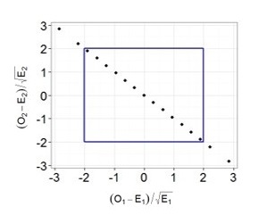
Now the fun part. Suppose that we decided to repeat 100 throws many times, and each time we recorded the observed frequencies of eagles and tails, calculated the required indicators (the difference between the observed and expected frequencies, divided by the root of the expected frequency) and, as in the previous example, plotted them on a graph.
It is easy to see that now all the points are aligned in one line. The thing is that in the case of a coin, our terms are not independent, knowing the total number of throws and the number of tails, we can always accurately determine the dropped number of eagles and vice versa, therefore we cannot say that our two terms are two independent random quantities. You can also make sure that all points will always always lie on one straight line: if we had 30 eagles, then there were 70 tails, if 70 eagles, then 30 tails, etc. Thus, despite the fact that there were two terms in our formula, we will use the Chi-square distribution with one degree of freedom to calculate p-value! So we finally got to the moment when we needed to subtract the unit. If we tested the hypothesis that Since our dice with six faces is honest, we would use a Chi-square distribution with 5 degrees of freedom. After all, knowing the total number of throws and the observed frequency of loss of any five faces, we can always determine exactly what the number of drops of the sixth face equals.
Everything falls into place
Now, armed with this knowledge, back to the t-test:
we have the standard error in the denominator, which is the sample standard deviation divided by the root of the sample size. The calculation of the standard deviation includes the sum of the squares of the deviations of the observed values from their average value - that is, the sum of several random positive values. But we already know that the sum of the squares of n random variables can be described using the chi-square distribution. However, despite the fact that we have n terms, this distribution will have an n-1 degree of freedom, since knowing the sample average and n-1 elements of the sample, we can always precisely specify the last element (hence this explanation about the average and n-1 elements needed to uniquely identify n elements)! It turns out that in the denominator of t-statistics we have hidden the chi-square distribution with n-1 degrees of freedom, which is used to describe the distribution of the sample standard deviation! Thus, the degrees of freedom in the t-distribution are actually taken from the chi-square distribution, which is hidden in the t-statistic formula. By the way, it is important to note that all the above considerations are true if the trait under study has a normal distribution in the general population (or the sample size is large enough), and if we really had the goal of testing the hypothesis of the average value of growth in the population, perhaps it is more reasonable to use a nonparametric criterion.
A similar logic for calculating the number of degrees of freedom is preserved when working with other tests, for example, in regression or variance analysis, the thing is in random variables with the Chi-square distribution, which are present in the formulas for calculating the relevant criteria.
Thus, in order to correctly interpret the results of statistical studies and to understand where all the indicators that we get when using even such a simple criterion as a single-sample t-test arise, any researcher needs to understand well what mathematical ideas underlie statistical methods.
Online statistics courses: explain complex topics in simple language
Based on the experience of teaching statistics at the Institute of Bioinformatics , we had the idea to create a series of online courses devoted to data analysis, in which the most important topics will be explained in an accessible form for each, understanding of which is necessary for the confident use of statistical methods in solving various problems. In 2015, we launched the Fundamentals of Statistics course , to which about 17 thousand people have signed up today, three thousand students have already received a certificate of successful completion, and the course itself has been awarded the EdCrunch Awards and recognized as the best technical course. This year, on the stepik.org platform , the continuation of the Basics of Statistics course has started . Part two, in which we continue our acquaintance with the basic methods of statistics and analyze the most complex theoretical issues. By the way, one of the main topics of the course is the role of the Pearson Chi-square distribution in testing statistical hypotheses. So if you still have questions about why we subtract the unit from the total number of observations, we are waiting for you on the course!
It is also worth noting that theoretical knowledge in the field of statistics will definitely be useful not only to those who use statistics for academic purposes, but also to those who use data analysis in applied fields. Basic knowledge of statistics is simply necessary to master the more complex methods and approaches that are used in the field of machine learning and Data Mining. Thus, successfully completing our introduction to statistics courses is a good start in data analysis. Well, if you are seriously thinking about acquiring data skills, we think you may be interested in our online data analysis program, which we wrote about in more detail here. The statistics courses mentioned are part of this program and will allow you to smoothly immerse yourself in the world of statistics and machine learning. However, everyone can take these courses without deadlines, even outside the context of a data analysis program.